Question 1:

• Note that u(2,8)=(2+2)(8+1)=36. Thus, we must solve (X+2)(Y+1)=36 for Y. We get XY+2Y+X+2=36. Hence Y(X+2)=34-X which implies Y=(34-X)/(X+2). Alternatively, XY+2Y+X+2=36. Hence Y(X+2)=36-(X+2). Thus, Y=36/(X+2)-1. This curve is indicated below.
  

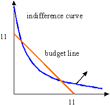
• As can be seen in the graph, the indifference curve contains consumption bundles that are in the budget set. In fact, strictly higher utility level can also be obtained.
• The partial derivatives with respect to X and Y are given by Y+1 and X+2, respectively. Thus, the MRS(X,Y)=-(Y+1)/(X+2).
• If the MRS is equal to the slope of the budget line then we get -(Y+1)/(X+2)=-1. This simplifies to X+2=Y+1, i.e.,
• The equation of the budget line is X+Y=11.
• Substituting Y=X+1 in X+Y=11 yields 2X+1=11. Thus, X=5 and Y=6.

Question 2:

• As indicated (25,0) and (16,4) give a utility of 20. The other points are (9,8), (4,12), (1,16), (0,20).
  
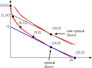
• If the drawing is sufficiently accurate, the solution should be 16. Note that the indifference curves are red and the budget line is blue in the graph.
• Some points that result in a utility level of 25 are (0,25), (1,21), (4,17), (9,13), (16,9), (25,5).
• The new optimal choice is (16,9) (the new budget line is gray). Note that the level of consumption of nuts does not change. The reason is that the MRS is given by MRS=-2/x₁^1/2. The price ratio is -1/2. Thus, MRS=-1/2 implies 2/x₁^1/2=1/2 and hence x₁=16, independent of the consumer's income.
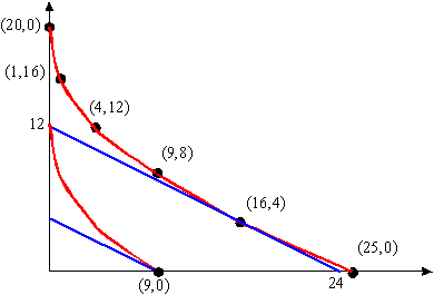
• The slope of the indifference curve at (9,0) is -2/3 (see the graph below or use the above MRS).
• The slope of the budget line is -1/2.
• At this point the indifference curve is steeper.
• No, as the graph below indicates, (9,0) is the optimal choice.

Question 3: Recall that at an optimal choice the MRS must be equal to the slope of the budget line if the optimal consumption is interior (no boundary solution) and if preferences have convex weakly preferred sets and are monotonic. Since (2,4) is not a boundary solution we can therefore conclude that the MRS(2,4)=-p₁/p₂=-3/2.

In the second case we have a boundary optimum. Hence, we cannot conclude that the MRS is equal to the slope of the budget line.

Question 4:

• The preferences are convex and monotone. Thus, If the price ratio is equal to the MRS then we can have an interior optimum. The MRS is -1/4. Thus, the price ratio must be -1/4. If you make the graph, then you will see that the budget line at this price ratio coincides with an indifference curve.
• If the -p₁/p₂ is not equal to -1/4 then there will be boundary optima. In particular, one can check by means of a graph that -p₁/p₂<-1/4 implies that the consumer chooses x₁=0. Otherwise, if -p₁/p₂>-1/4 we will have x₂=0 for the optimal consumption choice.

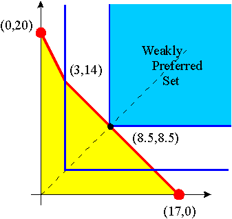
Question 5: Recall that the indifference curves are L-shaped (blue in the graph) and have a kink at the 45° axis, as indicated in the graph. The optimal choice is therefore the intersection point between the 45° axis and the budget line. The optimal consumption choice is (8.5,8.5).

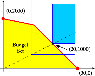
• The budget line is 2x₁+x₂=m=1.5. Thus, (0.5,0.5) is optimal.
• Now the budget line is 2x₁+x₂=2. Thus, (1,0) is optimal. Note that the MRS is equal to the slope of the budget line although we have a boundary optimum. Specifically, there exist examples such as this one, where at a boundary optimum the MRS is equal to the slope of the budget line. However, there are also cases of boundary optima (as in the last part of this question) where the two are not the same.
  
• The budget line is 2x₁+x₂=3. Thus, (2,-1) solves the two equations. This, however, cannot be an optimal consumption choice. Thus, we must have a boundary optimum at which the MRS is not equal to -p₁/p₂. The two candidates are (1.5,0) and (0,3). The utilities are log(1.5)+1.5 and log(3), respectively. One can easily check that the first utility is higher. Thus, (1.5,0) is optimal.
• The consumption of good 2 decreased from 0.5 to 0 when income was increased from 1.5 to 2). Goods with this property will be defined later in this class as inferior goods.

Question 7: You will find the main ideas for solving this question in your notes from the lecture of Wed., February 7.

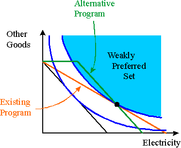
The black line in the graph is the budget line without any program. The red line in the graph is the budget line with the existing program. In order to find the budget line for the alternative program, note that it must look like the budget line in Figure 2.6 of the textbook. There must be a part where the line is horizontal that corresponds to the amount of electricity which is provided for free. After that, the budget line must have the same slope as the black budget line. Thus, we must determine the length of the flat part of the budget line.

Recall that the government should spend the same amount of money in both cases. Thus, intuitively the budget line for the alternative program must go through the optimal consumption bundle on the red budget line (indicated by a black dot). This insight allows us to construct the green budget line. Formally, this can shown as follows (c.f., Section 5.6 of the textbook).

Denote the optimal consumption bundle on the red line by (x₁*,x₂*). Then the government pays S=sx₁* as a subsidy. The budget line of the alternative program must therefore be of the form p₁x₁+x₂=m+S. In addition p₁x₁>=S must hold as the subsidy S must be used on electricity only (cf., the discussion on food stamps in class). Now recall that (x₁*,x₂*) is on the red line. Thus, (p₁-s)x₁*+x₂*=m. This is equivalent to p₁x₁*+x₂*=m+sx₁* which is the same as p₁x₁*+x₂*=m+S. In addition, p₁x₁*>S as one can see in the graph. However, this means that (x₁*,x₂*) is also on the green budget line.

It can be seen in the graph that the a part of the green budget line lies in the interior of the weakly preferred set for (x₁*,x₂*). Thus, the consumer is better off under the alternative program. Secondly, it can be seen from the graph that the consumption of good 1 is lower under the alternative program. In particular, for all points on the part of the green budget line which is inside the weakly preferred set, the consumption of good 1 is lower than x₁*.

To the title page