Stein's (1956) celebrated shrinkage results imply that one can improve upon
![]() in Gaussian regression problems with parametric dimension
in Gaussian regression problems with parametric dimension
![]() by shrinking
by shrinking ![]() toward some fixed point, thereby
trading bias for variance reduction. Judge and Bock (1978) treat this
subject in some detail from an econometric standpoint. One might
characterize this as statistical stoicism - through restraint, self-discipline
and temperance we achieve the noble purpose of reduced mean square error.
For others, it may be interpreted as a form of Bayesian parsimony.
toward some fixed point, thereby
trading bias for variance reduction. Judge and Bock (1978) treat this
subject in some detail from an econometric standpoint. One might
characterize this as statistical stoicism - through restraint, self-discipline
and temperance we achieve the noble purpose of reduced mean square error.
For others, it may be interpreted as a form of Bayesian parsimony.
We have no quarrel with such philosophies. They are fine for those who, like La Fontaine's ant, prefer to toil all summer to prepare for the hardships of winter. But who speaks out for the profligacy of the grasshopper, for gluttony and reckless abandon? Can such ideas have a place in the dismal annals of econometrics? We beg the gentle reader's momentary indulgence to consider the following foolishly profligate estimator:
Augment the p-columns of the initial design matrix X, by q randomly generated columns, D. Let, and consider estimating the augmented model by ordinary least squares,

and denote the familiar Eicker-White covariance matrix estimator for
by

where
and
. Finally, let
, so
, and define the GMM estimator of
, by solving

yielding,

This may appear to be the recipe of some demented sack-guzzler, but there is method in the madness. Our first result shows that we are not trading bias for variance reduction as in Stein estimation.
![]()
Proof: The argument is essentially that of Kakwani(1967); see also the treatment in Schmidt(1976). Fix Z and write
![]()
Observe that ![]() is an even function of u, that is u and -u
yield the same
is an even function of u, that is u and -u
yield the same ![]() . Since by assumption u and -u have the same
distribution, it follows that
. Since by assumption u and -u have the same
distribution, it follows that ![]() and
and
![]() have the same distribution.
And the result then follows by unconditioning on Z.
have the same distribution.
And the result then follows by unconditioning on Z.
We can conclude from this result that any improvement in mean squared error
acheived by ![]() must be purely a matter of variance reduction. Since for
Gaussian F it is well known that
must be purely a matter of variance reduction. Since for
Gaussian F it is well known that ![]() is minimum variance unbiased
we obviously must narrow the class of F's to exclude this case. Our
next result which is an immediate corollary of Theorem 2.2 of
Koenker, Machado, Skeels, and Welsh(1994), henceforth KMSW,
specifies the class of distributions for which we may expect
an improvement.
is minimum variance unbiased
we obviously must narrow the class of F's to exclude this case. Our
next result which is an immediate corollary of Theorem 2.2 of
Koenker, Machado, Skeels, and Welsh(1994), henceforth KMSW,
specifies the class of distributions for which we may expect
an improvement.
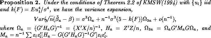
The first term in this variance expansion is familiar,
it is the variance that would result had we used the true ![]() .
The second term which is of order
.
The second term which is of order ![]() may be attributed to
the ``heteroscedasticity correction'' of the GMM estimator and
is probably less so.
It is easy to see that the
matrix
may be attributed to
the ``heteroscedasticity correction'' of the GMM estimator and
is probably less so.
It is easy to see that the
matrix ![]() is positive definite and consequently for
distributions with kurtosis greater than 5, the Falstaff estimator,
is positive definite and consequently for
distributions with kurtosis greater than 5, the Falstaff estimator, ![]() ,
has strictly smaller asymptotic covariance matrix, to order
,
has strictly smaller asymptotic covariance matrix, to order ![]() than the Gauss-Markov estimator
than the Gauss-Markov estimator ![]() .
.
Of course, for Gaussian F and other distributions with modest kurtosis the
second term contributes a positive component and consequently the ![]() ``correction for heteroscedasticity'' is counter-productive. This degradation
in performance at the Gaussian model is hardly surprising since classical
sufficiency arguments as in Rothenberg(1984) imply such a loss is inevitable.
``correction for heteroscedasticity'' is counter-productive. This degradation
in performance at the Gaussian model is hardly surprising since classical
sufficiency arguments as in Rothenberg(1984) imply such a loss is inevitable.
Intuitively, we would expect that ignoring the fact that our observations
are homoscedastic couldn't help us. We should be punished for ignoring
relevant information. Shouldn't we?
How then do we gain from the profligate behavior
of the Falstaff estimator? How can estimating an artificially expanded
model and then correcting for heteroscedasticity in an iid error model
conceivably increase the precision of our estimates?
To explore these questions we begin by considering the particularly simple
special case of estimating a scalar location parameter. Since in this
case X = 1 an n-vector of ones, the form of ![]() is especially
simple:
is especially
simple: ![]() ,
, ![]() , and therefore
, and therefore ![]() , the
number of augmented columns in D. Thus our expansion reduces in this
case to
, the
number of augmented columns in D. Thus our expansion reduces in this
case to
![]()
In the next section we report on a small monte-carlo experiment designed to evaluate the accuracy of this expansion for moderate sample sizes. What is the Falstaff estimator doing in this simple location context? The Falstaff estimator of location may be expressed as
![]()
Obviously, if ![]() is proportional to the identity matrix and
D is orthogonal to X then
is proportional to the identity matrix and
D is orthogonal to X then
![]() . However, generally, all the coordinates of
. However, generally, all the coordinates of
![]() contribute to
contribute to ![]() . If
. If ![]() converges in probability
to a nonstochastic matrix, the iid error assumption ensures that the limit
is proportional to the identity.
This simply restates the obvious fact that if
converges in probability
to a nonstochastic matrix, the iid error assumption ensures that the limit
is proportional to the identity.
This simply restates the obvious fact that if ![]() is consistent
as it would be in the present circumstances if q were fixed, then the Falstaff
improvement vanishes as
is consistent
as it would be in the present circumstances if q were fixed, then the Falstaff
improvement vanishes as ![]() . Whether there may
be some scope for asymptotic improvement if the sequence of
. Whether there may
be some scope for asymptotic improvement if the sequence of ![]() matrices
could be chosen to preserve a stochastic contribution from
matrices
could be chosen to preserve a stochastic contribution from ![]() remains an open question.
remains an open question.