
e-TA 9: Monte Carlo Simulation, Nonlinear Regression and and Simultaneous Equations Models
Welcome to a new e-Tutorial. The first part of the tutorial is useful for the first part of problem set 3. It will help you to understand details of Granger and Newbold (1974). This time we focus on Monte Carlo Simulation and Nonlinear Regression. I introduce these two topics in form of examples connected to Econ 508 syllabus. For the Monte Carlo, we use the Granger-Newbold experiment on spurious regression as an example. For the Nonlinear Regression, we give examples of how to correct autocorrelated errors (NLS and Cochrane-Orcutt).1
Monte Carlo Simulation:
In the Granger-Newbold (1974) experiment, the econometrician has a bivariate model as follows:
\[ y_{t} = b_{0} + b_{1} x_{t} + e_{t} \] where \[ y_{t} = y_{t-1} + u_{t} \] \[ x_{t}= x_{t-1} + v_{t} \] \(u_{t}\) and \(v_{t}\) are identically independently distributed. Hence, each variable has a unit root, and their differences, \(y_{t}-y_{t-1}=u_{t}\) and \(x_{t}-x_{t-1}=v_{t}\), are pure noise. However, as you regress \(y_{t}\) on \(x_{t}\), you may obtain significant linear relationship based on conventional OLS and t-statistics, contrary to your theoretical expectations.
Let’s replicate the experiment. The algorithm is as follows: - generate the errors of each series as random normal variables with mean zero, variance 1, and size 100 - build the series - regress the series - plot the series - plot the fitting line and show the t-statistic of its slope
This corresponds to a single loop of the experiment, but it is already enough to show the nuisance. If you wish, you can go ahead and repeat this loop B times and check how many times you get significance.
Below I provide the routine for one iteration of the simulation for Stata, which can also also be accessed at the Econ 508 web page, Routines, under the name gn.do.
Stata Code:
clear all
set obs 100
gen t=_n
gen u=invnorm(uniform())
gen y=u if t==1
replace y=y[_n-1]+u if t>1
gen v=invnorm(uniform())
gen x=v if t==1
replace x=x[_n-1]+v if t>1
regress y x
twoway (line y t) (linex t), title("Fig. 1: Y and X Time Series")
twoway(scatter y x) (lfit y x), title("Fig. 2: Y fitted on X")
Since this is a simulation it is very important to set seed at the very begining in order to allow reproducible results. The figures of the iteration above using set seed 1 are:
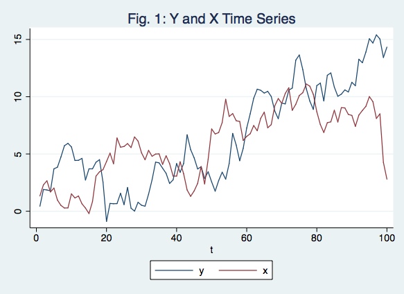
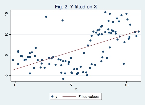
Note that the result of this single simulation you get a very significant t-statistic even though there’s no relation between the series.
Nevertheless, as many times you run as more convinced you will be
that in a large proportion of the cases the t-statistics will be very
significant, meaning that you have spurious regression in many cases.
Nonlinear Regression:
We explain nonlinear regression through the data sets of the problem
set 3. You can download them in ASCII format by clicking in the
respective names: cob1.txt and cob2.txt. Save them in your preferred
location. Then I suggest you to open the files in Notepad (or another
text editor) and type the name of the variable “year” in the first row,
first column, i.e. before the variable “w”. Use
The problem:
Suppose you have the following equation:
\[ Q_{t}= a_{1} + a_{t} p_{t-1}+ a_{3} z_{t} + u_{t} \]
and you suspect the errors are autocorrelated. The first you need to explain why \(p_{t}\) cannot be considered exogenous. Please also explain the consequences of applying OLS estimators in the presence of autocorrelated disturbances.
Testing for the presence of autocorrelation:
Next you need to test for the presence of autocorrelation. You already saw a large menu of options for that. Here I suggest the use of the Breusch-Godfrey test:
Background: Here you are assuming that \(e_{t}\) is a white noise process and
\[ Q_{t}= a_{1} + a_{2} p_{t-1}+ a_{3} z_{t} + u_{t} \] \[ u_{t}= b_{1} u_{t-1} + b_{2} u_{t-2} + ...+ b_{p} z_{t-p} + e_{t} \]
You wish to test whether any of the coefficients of lagged residuals is different than zero. Your null hypothesis is no autocorrelation, i.e., \(b_{1}=b_{2}=...=b_{p}=0\). For example, to test for the presence of autocorrelation using 1 lag (AR(1)), do as follows:
*Run an OLS in your original equation:
  gen t=_n
  tsset t
  reg q L.p z
      Source |       SS       df       MS              Number of obs =     199
-------------+------------------------------           F(  2,   196) =  228.23
       Model |  2990.56983     2  1495.28492           Prob > F      =  0.0000
    Residual |  1284.14854   196  6.55177829           R-squared     =  0.6996
-------------+------------------------------           Adj R-squared =  0.6965
       Total |  4274.71838   198  21.5894867           Root MSE      =  2.5596

------------------------------------------------------------------------------
           q |      Coef.   Std. Err.      t    P>|t|     [95% Conf. Interval]
-------------+----------------------------------------------------------------
           p |
         L1. |   .9422375   .0441069    21.36   0.000     .8552526    1.029222
             |
           z |   .4860205   .1735232     2.80   0.006     .1438082    .8282328
       _cons |  -.3871965   .6114427    -0.63   0.527    -1.593048    .8186548
------------------------------------------------------------------------------
*Obtain the estimated residuals:
predict uhat, resid- Regress the estimated residuals on the explanatory variables of the original model and lag of residuals:
regress uhat L.p z L.uhat
      Source |       SS       df       MS              Number of obs =     198
-------------+------------------------------           F(  3,   194) =   49.72
       Model |  553.712546     3  184.570849           Prob > F      =  0.0000
    Residual |   720.19318   194  3.71233598           R-squared     =  0.4347
-------------+------------------------------           Adj R-squared =  0.4259
       Total |  1273.90573   197  6.46652653           Root MSE      =  1.9267

------------------------------------------------------------------------------
        uhat |      Coef.   Std. Err.      t    P>|t|     [95% Conf. Interval]
-------------+----------------------------------------------------------------
           p |
         L1. |   .1023098   .0342883     2.98   0.003     .0346841    .1699354
             |
           z |    .032555    .130972     0.25   0.804    -.2257568    .2908667
             |
        uhat |
         L1. |   .6768817   .0554303    12.21   0.000     .5675582    .7862052
             |
       _cons |  -1.110674   .4715092    -2.36   0.019    -2.040617    -.180732
------------------------------------------------------------------------------
*From the auxiliary regression above, obtain the R-squared and multiply it by number of included observations:
   scalar nR2=e(r2)*e(N)
   dis nR2
86.062164This nR2 may be compared with a \(\chi^{2}_{1}\) distribution. If you need to test autocorrelation using \(p\) lags, compare your statistic with a \(\chi^{2}_{p}\). Hint: Be parsimonious - don’t push the data too much, and try to use at most 4 lags. However, observe that the first lag is enough to detect autocorrelation here.
Correcting the Model:
After you detect autocorrelation, you need to correct it. Let’s see how it works in our data. Suppose we have obtained the following AR(1) autocorrelation process:
\[ Q_{t}= a_{1} + a_{2} p_{t-1}+ a_{3} z_{t} + u_{t} \; \; \;(1) \] \[ u_{t}= b_{1} u_{t-1} + e_{t} \; \; \; (2) \]
where \(e_{t}\) is white noise. Now generate the lag of equation (1):
\[ Q_{t-1}= a_{1} + a_{2} p_{t-2}+ a_{3} z_{t-1} + u_{t-1} \; \; \;(3) \]
and substitute (3) into the equation (2):
\[ u_{t}= b_{1} (Q_{t-1}- a_{1} - a_{2} p_{t-2}- a_{3} z_{t-3}) + e_{t} \; \; \;(4) \]
Substituting equation (4) into the equation 1 will give you an autocorrelation-corrected version of your original equation:
\[ Q_{t}= b_{1} Q_{t-1} + a_{1} (1 - b_{1}) + a_{2} p_{t-1}+ a_{3} z_{t} - b_{1} a_{2} p_{t-2} - b_{1} a_{3} z_{t-1} + e_{t} \; \; \;(5) \]
This corrected model contain multiplicative terms in the
coefficients, and therefore need to be re-estimated by Non-linear Least
Squares (NLS). To implement Non-linear Least Squares you can program
the nls function to estimate your model:
 program define nlg
    if "`1'"  ==  "?"  {
        global S_1   "rho  a1  a2  a3"
        global rho =.5
        global a1  =.5
        global a2  =.5
        global a3  =.5
        exit
    }
    replace `1' = $rho*L.q + $a1*(1-$rho) + $a2*L.p + $a3*z - $rho*$a2*L2.p  - $rho*$a3*L.z
end
In the program above:
Line 1: corresponds to the name of the program (g is the name, nl is the method)
Line 2: corresponds to the expression to
be created, in which you are going to insert your regression equation
Line 3: corresponds to the vector of
parameters to be calibrated. In the equation (5) above, rho corresponds
to b1, while a1, a2, and a3 are themselves.
Lines 4-7: corresponds to the initial value of each parameters for the
calibration, The system will start with those values and them, using an
iterative process, it will try to converge to a final value value of
each parameter that optimizes the whole equation.
Lines 8-9: used to separate different parts within the same program.
Line 10: corresponds to your equation (5), using the parameters created in S_1
Line 11: finishes your program.
Ok. After you have created the program g, you need to run it. Attempt to one detail: the program does not work in the presence of missing values. As you have generated lags, you also have lost the first 2 observations. Thus, you need to restrict your optimization problem to the existing observations.
nl g q if year>1960.25 Iteration 0: residual SS = 2709.559
Iteration 1: residual SS = 746.0734
Iteration 2: residual SS = 713.0033
Iteration 3: residual SS = 712.8309
Iteration 4: residual SS = 712.8309
Iteration 5: residual SS = 712.8309
Source | SS df MS Number of obs = 198
-------------+------------------------------ F( 3, 194) = 322.72
Model | 3557.38751 3 1185.79584 Prob > F = 0.0000
Residual | 712.830903 194 3.6743861 R-squared = 0.8331
-------------+------------------------------ Adj R-squared = 0.8305
Total | 4270.21842 197 21.6762356 Root MSE = 1.916869
Res. dev. = 815.5331
(g)
------------------------------------------------------------------------------
q | Coef. Std. Err. t P>|t| [95% Conf. Interval]
-------------+----------------------------------------------------------------
rho | .6691202 .0533881 12.53 0.000 .5638246 .7744158
a1 | -1.458362 .7274565 -2.00 0.046 -2.893101 -.0236235
a2 | 1.025829 .0251139 40.85 0.000 .9762975 1.07536
a3 | .5902033 .292248 2.02 0.045 .013812 1.166595
------------------------------------------------------------------------------
* Parameter a1 taken as constant term in model & ANOVA table
(SEs, P values, CIs, and correlations are asymptotic approximations)
That is it. The output should give you the requested elements to calculate equation (5) - the model adjusted for autocorrelation. Similar result can be obtained through the Cochrane-Orcutt method. In STATA, you can obtain that as follows:
prais q L.p z, corcThis will give you the adjusted coefficients of each explanatory variable, plus the Durbin-Watson statistic before and after the correction. Compare the Cochrane-Orcut results with the NLS results, and see how similar they are. Then compare both NLS and Cochrane-Orcutt with the naive OLS from question 1, and draw your conclusions.
Second half: Problem set 3
For the first question you need to run the following system by OLSSuppose you have the following equation:
Suppose you have the following equation:
\[ Q_{t}= a_{1} + a_{2} p_{t-1}+ a_{3} z_{t} + u_{t} \; \; \; \; \; (Supply) \] \[ p_{t}= b_{1} + b_{2} Q_{t}+ b_{3} w_{t} + v_{t} \; \; \; \; \; (Demand) \]
*Supply equation:
reg q L.p z
*Demand equation:
regp q w
.   *Supply equation:

.   regress  q  L.p   z

      Source |       SS       df       MS              Number of obs =     199
-------------+------------------------------           F(  2,   196) =  228.23
       Model |  2990.56983     2  1495.28492           Prob > F      =  0.0000
    Residual |  1284.14854   196  6.55177829           R-squared     =  0.6996
-------------+------------------------------           Adj R-squared =  0.6965
       Total |  4274.71838   198  21.5894867           Root MSE      =  2.5596

------------------------------------------------------------------------------
           q |      Coef.   Std. Err.      t    P>|t|     [95% Conf. Interval]
-------------+----------------------------------------------------------------
           p |
         L1. |   .9422375   .0441069    21.36   0.000     .8552526    1.029222
             |
           z |   .4860205   .1735232     2.80   0.006     .1438082    .8282328
       _cons |  -.3871965   .6114427    -0.63   0.527    -1.593048    .8186548
------------------------------------------------------------------------------

.   *Demand equation:

.   regress  p  q  w

      Source |       SS       df       MS              Number of obs =     200
-------------+------------------------------           F(  2,   197) =   86.62
       Model |  1603.33345     2  801.666725           Prob > F      =  0.0000
    Residual |  1823.27998   197  9.25522835           R-squared     =  0.4679
-------------+------------------------------           Adj R-squared =  0.4625
       Total |  3426.61344   199   17.219163           Root MSE      =  3.0422

------------------------------------------------------------------------------
           p |      Coef.   Std. Err.      t    P>|t|     [95% Conf. Interval]
-------------+----------------------------------------------------------------
           q |  -.4854016   .0497097    -9.76   0.000     -.583433   -.3873702
           w |   4.119399   .3521172    11.70   0.000     3.424996    4.813802
       _cons |   8.585394   .6385986    13.44   0.000     7.326027    9.844761
------------------------------------------------------------------------------
and you suspect the errors are autocorrelated. The first you need to explain why \(p_{t}\) cannot be considered exogenous. Please also explain the consequences of applying OLS estimators in the presence of autocorrelated disturbances.
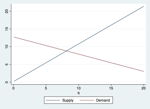
For the graph, first consider the equations in the steady state. Then use the last observations values z and w. Finally plot those two equations in a single cartesian graph. Don’t forget to find the equilibrium price and quantity. Compare with your graph. Check if there’s convergence in the graph (see Prof. Koenker class notes).
* Get coefficients for Supply equation
qui: reg q L.p z
scalar a1=_b[_cons]
scalara2=_b[L.p]
scalara3=_b[z]
* Get coefficients for demand equation
qui: regp q w
scalarb1=_b[_cons]
scalarb2=_b[q]
scalarb3=_b[w]
preserve
* Save last values of series
qui: sum year
keep if year==r(max)
scalarw=w
scalarz=z
clear
set obs 200
gen q = _n/10
genP_s = (q)/a2 - (a1 + a3*z)/a2
genP_d = b2*(q) + (b1 + b3*w)
twoway (line P_s q) (lineP_d q), legend(label(1 "Supply") label(2 "Demand"))
restore
Note: The commands preserve saves the data as it is in the temporary memory of the computer. After modifying it, deleting observations, deleting the whole thing, creating new data, etc. we can return to the data as it was at the point when we input preserve by typing restore. Note that you can restore once, so if you want to modify the current data and then return to how the data is at this point then you will have to type preserve again.
Hausman Test
Here you can use the Hausman specification test you have saw in the Lecture. Make sure to explain the null and the alternative hypothesis, and describe how the test is computed. The choice of instruments is crucial: you need to select instruments that are exogenous, orthogonal to errors, but correlated with included variables. In Stata, you can calculate the Hausman test as follows:* 2SLS with full set of instruments:
ivreg q (L.p =your instruments l.w)z
matrix bFull=e(b)
matrixvarFull=e(V)
estimates store Fm
* 2SLS with reduced set of instruments:ivregq (L.p =your instruments)z
matrixbRedux=e(b)
matrixvarRedux=e(V)
estimates store Rm
* Hausman Specification Test by hand:
matrixOmega=varRedux-varFull
matrixOmegainv=syminv(Omega)
matrixq=bFull-bRedux
matrixDelta=q*Omegainv*q'
matrixlist Delta
* Hausman Stata command:
hausman Fm Rm
References
Granger, C., and P. Newbold (1974): “Spurious Regression in Econometrics,” Journal of Econometrics, 2, 111-120
Please send comments to bottan2@illinois.edu or srmntbr2@illinois.edu↩