
e-TA 8: Unit Roots and Cointegration
Welcome to this new issue of e-Tutorial. We focus now on time series models, with special emphasis on the tests of unit roots and cointegration. We would like to remark that the theoretical background given in class is essential to proceed with the computational exercise below. Thus, I recommend you to study Prof. Koenker’s Lectures 8 and 9 as you go through the tutorial.1
Data
The first thing you need is to download the updated Thurman and Fisher (1988) data, called eggs.csv from the Econ 508 web site. Save it in your preferred directory and open the data:
  cd "Your working directory"
  insheet using eggs.csv, clear
The next step is to declare chickens and eggs as time series:
tsset yearUnit Root: Augmented Dickey-Fuller Test
At first, it is important that you to sketch the ADF test, explaining the NULL and the ALTERNATIVE hypotheses.
ADF Test in Stata: Once
again, I recommend you to show explicitly what are the NULL and
ALTERNATIVE hypotheses of this test, and the regression equations you
are going to run. Then, using the STATA, you have two ways to perform
the test:
- using the dfuller command , or
- using OLS (but checking for significance in the Dickey-Fuller tables)
(a) models with intercept and trend;
(b) models with intercept, but without trend;
(c) models without both intercept and trend.
A simple example of ADF:
a) Models including constant and trend: For example, using 1 lag in the chicken series, you will have the following result
dfuller chic, regress trend lags(1)
Augmented Dickey-Fuller test for unit root         Number of obs   =        73

                               ---------- Interpolated Dickey-Fuller ---------
                  Test         1% Critical       5% Critical      10% Critical
               Statistic           Value             Value             Value
------------------------------------------------------------------------------
 Z(t)             -1.678            -4.099            -3.477            -3.166
------------------------------------------------------------------------------
MacKinnon approximate p-value for Z(t) = 0.7605

------------------------------------------------------------------------------
D.chic       |      Coef.   Std. Err.      t    P>|t|     [95% Conf. Interval]
-------------+----------------------------------------------------------------
        chic |
         L1. |  -.1143316   .0681419    -1.68   0.098    -.2502709    .0216077
         LD. |   -.097584   .1222598    -0.80   0.428    -.3414856    .1463176
      _trend |  -.2079985    138.481    -0.00   0.999      -276.47     276.054
       _cons |   47109.16   30968.52     1.52   0.133    -14671.35    108889.7
------------------------------------------------------------------------------
b) Models including constant but no trend: Same rationale, but adjusting the command to:
dfuller chic, regress lags(1)Augmented Dickey-Fuller test for unit root Number of obs = 73
---------- Interpolated Dickey-Fuller ---------
Test 1% Critical 5% Critical 10% Critical
Statistic Value Value Value
------------------------------------------------------------------------------
Z(t) -1.908 -3.548 -2.912 -2.591
------------------------------------------------------------------------------
MacKinnon approximate p-value for Z(t) = 0.3285
------------------------------------------------------------------------------
D.chic | Coef. Std. Err. t P>|t| [95% Conf. Interval]
-------------+----------------------------------------------------------------
chic |
L1. | -.114284 .0599086 -1.91 0.061 -.233768 .0051999
LD. | -.0976262 .1181335 -0.83 0.411 -.333236 .1379836
|
_cons | 47081.67 24802.08 1.90 0.062 -2384.52 96547.86
------------------------------------------------------------------------------
c) Models excluding both constant and trend: Idem, but adjusting the command to:
dfuller chic, noconstant regress lags(1)Augmented Dickey-Fuller test for unit root Number of obs = 73
---------- Interpolated Dickey-Fuller ---------
Test 1% Critical 5% Critical 10% Critical
Statistic Value Value Value
------------------------------------------------------------------------------
Z(t) -0.185 -2.611 -1.950 -1.610
------------------------------------------------------------------------------
D.chic | Coef. Std. Err. t P>|t| [95% Conf. Interval]
-------------+----------------------------------------------------------------
chic |
L1. | -.0011638 .0062782 -0.19 0.853 -.0136823 .0113546
LD. | -.1515686 .1167483 -1.30 0.198 -.3843581 .0812209
------------------------------------------------------------------------------
Those equations regard unit root tests for the chickens annual
series, using 1 lag. I recommend you to repeat these 3 processes for
lags 2,3,and 4 as well. After you complete this cycle for chickens, you
need to do the same cycle for eggs. At the end of both cycles, you will
have 24 regression outputs. If you prefer, you don't need to report all
output details, but rather concentrate on the ADF test statistics of
each equation. You can do that by ommiting the term "regress" on the
dfuller command.
Presenting your ADF results:
Think that you are writing an academic paper. Don't spend too much
space with intermediary results; concentrate instead on your final
conclusions, which can be paradoxical as you go through different
tetsting steps. By the end of the day you are expected to summarize
your main results in a table, and then to write a paragraph with
comments on the different results you can obtain when you
include/exclude trends/constants/lags for both chickens and eggs
series.
Cointegration: Engle-Granger Test
The first thing you should do always is to sketch the Engle-Granger test, explaining the NULL and the ALTERNATIVE hypotheses. :
Engle-Granger in Stata: The test can be done in 3 steps, as follows:
Pre-test the variables for the presence of unit roots (done above) and check if they are integrated of the same order
Regress the long run equilibrium model of chickens vs. eggs
regress chic egg
      Source |       SS       df       MS              Number of obs =      75
-------------+------------------------------           F(  1,    73) =    1.52
       Model |  2.9661e+09     1  2.9661e+09           Prob > F      =  0.2218
    Residual |  1.4261e+11    73  1.9536e+09           R-squared     =  0.0204
-------------+------------------------------           Adj R-squared =  0.0070
       Total |  1.4558e+11    74  1.9672e+09           Root MSE      =   44199

------------------------------------------------------------------------------
        chic |      Coef.   Std. Err.      t    P>|t|     [95% Conf. Interval]
-------------+----------------------------------------------------------------
         egg |  -6.228521   5.054826    -1.23   0.222    -16.30278    3.845734
       _cons |   446387.6   27575.93    16.19   0.000     391428.9    501346.4
------------------------------------------------------------------------------
Obtain the residuals.
predict residual, resPlot the residuals along time.
line residual year, title(Residuals vs. year)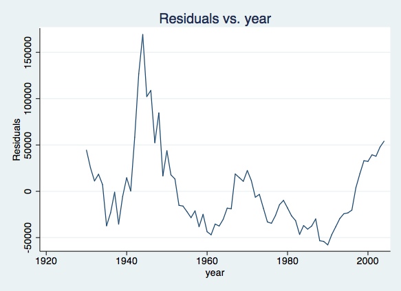
Graph the residuals against lagged residuals.
twoway (scatter residual L.residual) (lfit residual L.residual), title(Residuals vs. Lagged Residuals)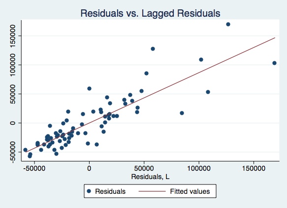
Plot also the residuals versus lagged residuals. Draw your conclusions
- Proceed with a unit root test on the residuals, i.e. test whether the residuals are \(I(0)\), as you have done the ADF test for unit roots on chickens and eggs. Consider lags 0 to 4, though. This is a residual-based version of the ADF test. The only difference from the traditional ADF to (this version of) the Engle-Granger test are the critical values. The critical values to be used here are no longer the same provided by Dickey-Fuller, but instead provided by Engle and Yoo (1987) and others (see approximated critical values in Table B.9, Hamilton 1994) HERE. This happens because the residuals above are not the actual error terms, but estimated values from the long run equilibrium equation of chickens against eggs.
Some authors (e.g., Enders, 1995) consider a fourth step, consisting in the estimation of error-correction models and checking of models adequacy. However, you are not required to do that for the purposes of the problem set 3.
At the end of the test, please provide a table summarizing your results. Comment your findings.
Cointegration: Johansen Test
Again we recommend you to sketch the Johansen test, explaining the
NULL and the ALTERNATIVE hypotheses.
Stata already has a function for testing for cointegration: vecrank
After defining data as time series, write:
vecrank egg chicThe code above refers to the case including trend and intercept, and the appropriate critical values should be used. Note that the theoretical background here is essential, given that you need to interpret the eigenvalues and calculate the test statistic by yourself, before to draw your conclusions.
Please send comments to bottan2@illinois.edu or srmntbr2@illinois.edu↩
Comments on Unit Root Tests:
Unit root tests are very sensitive to the number of included lags and/or constant and trends. That’s the reason by which we are asking you to show all ADF statistics in the table above. Very likely, some of the results will indicate the presence of unit root while others will not.
How to make a general conclusion on the test results with so many models available? Johnston & DiNardo (1997, p.226), for example, mention that one of the objectives of including lags is to achieve white noise residuals. Other authors recommend the use AIC or SIC in the model selection.
It is quite simple to calculate information criteria in ADF tests. Each output of dfuller corresponds to a linear regression on the lags, constant, and/or trend of the series. From OLS regression, you recover the sample size, the RSS, and the # of parameters requested to calculate SIC or AIC, plus the original ADF statistic. But remember to use the Dickey-Fuller critical values.