e-TA 5: Delta Method and Bootstrap Techniques
Welcome to e-Tutorial, your on-line help to Econ508. This issue provides an introduction on how to do the piratical works about the Delta-method and bootstrap in R. Hope this will be helpful for your further understanding of Prof. Koenker’s Lecture 5.1
Data Set
The data set used in this tutorial was borrowed from Johnston and DiNardo’s Econometric Methods (1997, 4th ed), but slightly adjusted for your needs. It is called AUTO2. You can download the data by visiting the Econ 508 web site (Data). As you will see, this adapted data set contains five series.
    use AUTO2, clear
    describe
obs: 128 AUTO2 adapted from Johnston and DiNard
vars: 5 11 Sep 2002 12:22
size: 2,560
------------------------------------------------------------------------------------
storage display value
variable name type format label variable label
------------------------------------------------------------------------------------
quarter float %9.0g Quarter of the observation
gas float %9.0g Log of per capita real expenditure on
price float %9.0g Log of the real price of gasoline and
income float %9.0g Log of per capita real disposable inco
miles float %9.0g Log of miles per gallon
------------------------------------------------------------------------------------
Sorted by:
As we did before we need to transform the data in “time series” first:
    gen t = _n
    label variable t "Integer time period"
    tsset t
time variable: t, 1 to 128
delta: 1 unit
Running a Dynamic Model with Quadratic and Multiplicative Terms
In the problem set 2, question 4, you are asked to run a linear regression model with non-linear transformation of variables. Suppose for a moment that you have in your hands a data set like the one used here (auto2.dta), and would like to estimate an equation similar to the problem set:
\[gas_{t} = b_{0} + b_{1} income_{t} + b_{2} price_{t} + b_{3} price_{t} ^2 + b_{4} (price_{t}*income_{t}) + u_{t}\]
first you need first to generate the quadratic and other terms as follows:
    gen price2= price^2
    gen priceinc= price*income
then regress:
regress gas income price price2 priceinc Source | SS df MS Number of obs = 128
-------------+------------------------------ F( 4, 123) = 117.59
Model | 1.45421455 4 .363553638 Prob > F = 0.0000
Residual | .38027632 123 .003091677 R-squared = 0.7927
-------------+------------------------------ Adj R-squared = 0.7860
Total | 1.83449087 127 .01444481 Root MSE = .0556
------------------------------------------------------------------------------
gas | Coef. Std. Err. t P>|t| [95% Conf. Interval]
-------------+----------------------------------------------------------------
income | -6.109449 2.750048 -2.22 0.028 -11.553 -.6658978
price | 3.090076 2.894747 1.07 0.288 -2.639898 8.82005
price2 | .2839261 .1693137 1.68 0.096 -.05122 .6190723
priceinc | 1.454257 .5879186 2.47 0.015 .290508 2.618006
_cons | -25.52231 11.8968 -2.15 0.034 -49.0713 -1.973312
------------------------------------------------------------------------------
Now, suppose you are asked to calculate the price elasticity of demand at different points of the sample. To do that you will need to:
- Obtain the coefficients of regression:
matrix B=get(_b)
matrix list BB[1,5]
income price price2 priceinc _cons
y1 -6.1094494 3.0900762 .28392614 1.4542568 -25.522308 - Extract the coefficients to scalars:
Or another way to do it: scalar b1=B[1,1] or scalar b1=_b[income]scalar b1=_coef[income]
scalarb2=_coef[price]
scalarb3=_coef[price2]
scalarb4=_coef[priceinc]
scalarb0=_coef[_cons]
scalarlist b1 b2 b3 b4 b0
iii. Calculate the elasticity at different:
gen elastpt=b2+2*b3*price+b4*income
summarize elastpt, detail elastpt
-------------------------------------------------------------
Percentiles Smallest
1% -.7897052 -.8065645
5% -.7665387 -.7897052
10% -.7234885 -.7795596 Obs 128
25% -.4959842 -.7698234 Sum of Wgt. 128
50% -.2754352 Mean -.3273864
Largest Std. Dev. .2598182
75% -.0774807 .0347935
90% -.0073602 .0391868 Variance .0675055
95% .0219321 .0460309 Skewness -.2600589
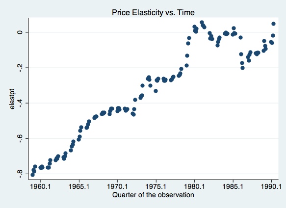
99% .0460309 .0555678 Kurtosis 1.835793 scatter elastpt quarter, xlabel(1960.1 (5) 1990.1) t1title(Price Elasticity vs. Time)
scatter elastpt gas, t1title(Price Elasticity vs. Gas Expenditure)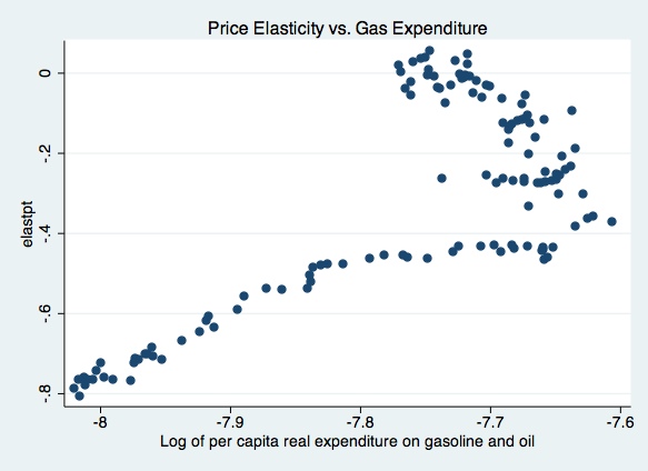
scatter elastpt price, t1title(Price Elasticity vs. Price)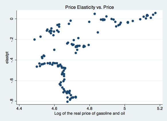
Tip for problem set 2, question 5.
For this question you should:
Interpret the implications of the model.
Calculate the price such that \([b_{2}+2*b_{3}*price+b_{4}*income] = -1 \) Given the formula of elasticity, and assuming \(income=x_{0}\), just find the optimal price. Call it \(p^{*}\).
Examine the partial residual plots
Finally, in the last part of the question 5 you are asked to estimate model 2 and to compute the revenue maximizing price level assuming \(income=\$30.000\) per year. This is a straightforward computation. The interesting part come with the application of the delta method and the bootstrap to achieve reasonable confidence intervals for the optimal price.
Delta-method and Bootstrap
Note that we obtained point estimates. To compute confidence intervals, you will need the Delta-method and/or Bootstrap. In the problem set you are asked to assume that \(income=\$30.000\) per year. For this e-ta, we will assume \(income=log(15)=2.708050\) approximately
Delta-method
For the problem set you are expected to sketch the Delta-method and calculate the derivatives by hand along with the computational routine below.
- Start running the full model again:
regress gas income price price2 priceinc
      Source |       SS       df       MS              Number of obs =     128
-------------+------------------------------           F(  4,   123) =  117.59
       Model |  1.45421455     4  .363553638           Prob > F      =  0.0000
    Residual |   .38027632   123  .003091677           R-squared     =  0.7927
-------------+------------------------------           Adj R-squared =  0.7860
       Total |  1.83449087   127   .01444481           Root MSE      =   .0556

------------------------------------------------------------------------------
         gas |      Coef.   Std. Err.      t    P>|t|     [95% Conf. Interval]
-------------+----------------------------------------------------------------
      income |  -6.109449   2.750048    -2.22   0.028      -11.553   -.6658978
       price |   3.090076   2.894747     1.07   0.288    -2.639898     8.82005
      price2 |   .2839261   .1693137     1.68   0.096      -.05122    .6190723
    priceinc |   1.454257   .5879186     2.47   0.015      .290508    2.618006
       _cons |  -25.52231    11.8968    -2.15   0.034     -49.0713   -1.973312
------------------------------------------------------------------------------
- Recall that you have stored those coefficients under the names b0, b1, b2 , b3, b4. Now you need to get the covariance matrix V of them:
    matrix V=get(VCE)
    matrix list V
symmetric V[5,5]
income price price2 priceinc _cons
income 7.5627648
price -6.5629988 8.3795596
price2 -.00833388 -.27004512 .02866714
priceinc -1.6166822 1.405926 .00149168 .34564825
_cons 30.88608 -33.229023 .62976256 -6.6089597 141.53396
- Next you need to input pstar:
  scalar pstar = -(1+b2+b4*ln(15))/(2*b3)
  scalar list pstar
pstar = -14.137967- And then you need to obtain the gradient vector with the partial derivatives of pstar (optimal price) with respect to each regressor, obeying the order of the covariance matrix:
\[G'= (\frac{\partial{p^{*}}}{\partial{cons}}, \frac{\partial{p^{*}}}{\partial{income}}, \frac{\partial{p^{*}}}{\partial{price}}, \frac{\partial{p^{*}}}{\partial{price2}}, \frac{\partial{p^{*}}}{\partial{price\_income}}) \]
In Stata the vector will be as follows (note that the backslashes separate each row of the vector):
  matrix G=( 0  \  -1/(2*b3)  \  (1+b2+b4*ln(15))/(2*b3*b3)  \  -ln(15)/(2*b3)  \  0)
  matrix list G
G[5,1]
c1
r1 0
r2 -1.7610213
r3 49.794522
r4 -4.7689342
r5 0 - The next step is to obtain the estimated variance of the optimal price, \(G'VG\):
   matrix GVG=G'*V*G
   matrix list
symmetric GVG[1,1]
c1
c1 175.19377- Then you can obtain the standard error by taking the square root of this scalar value:
   scalar sepstar=sqrt(el(GVG,1,1))
   scalar list sepstar
sepstar = 13.236079
That’s it. The variable sepstar is the standard error of pstar.
- The last step is to construct your confidence interval, and put the variables in levels, as follows:
   scalar CIupper=pstar + 1.96*sepstar
   scalar CIlower=pstar - 1.96*sepstar
   scalar list CIlower pstar CIupper
CIlower = -40.08068
pstar = -14.137967
CIupper = 11.804747
This will give you the confidence interval of the optimal price level. Observe that the results you obtained are for prices in logs. You can try to get the respective results in levels as well, but it is worth to think about whether you can do that directly or you need some additional step because of the non-linearity of the point estimate.
Bootstrap
You are expected to explain the various Bootstrap techniques in words (as if you are explaining for a non-econometrician), along with the complete understanding of the results provided by STATA.
In STATA, you can calculate parametric (Normal), percentiled, and bias corrected bootstrapped confidence intervals for the optimal price as follows:
 bs pr=(-1*(1+_b[price]+_b[priceinc]*ln(15))/(2*_b[price2])), reps(1000):
    reg gas income price price2 priceinc
Bootstrap replications (1000)
----+--- 1 ---+--- 2 ---+--- 3 ---+--- 4 ---+--- 5
.................................................. 50
.................................................. 100
.................................................. 150
.................................................. 200
.................................................. 250
.................................................. 300
.................................................. 350
.................................................. 400
.................................................. 450
.................................................. 500
.................................................. 550
.................................................. 600
.................................................. 650
.................................................. 700
.................................................. 750
.................................................. 800
.................................................. 850
.................................................. 900
.................................................. 950
.................................................. 1000
Linear regression Number of obs = 128
Replications = 1000
command: regress gas income price price2 priceinc
pr: -1*(1+_b[price]+_b[priceinc]*ln(15))/(2*_b[price2])
------------------------------------------------------------------------------
| Observed Bootstrap Normal-based
| Coef. Std. Err. z P>|z| [95% Conf. Interval]
-------------+----------------------------------------------------------------
pr | -14.13797 270.9505 -0.05 0.958 -545.1913 516.9153
------------------------------------------------------------------------------
Recall the generated statistic is in log form. A good question is whether you should present your Delta-method and Bootstrap confidence interval in logs or in levels... Think about it.
Appendix A: Partial Residual Plot Revisited
It is important to mention that all results presented here are based on a different data set (auto2.dta) than the data set used on the problem set 2 (gasnew.dat):
- Use the partial residual plot to check on the effect of the quadratic term. To obtain the partial residual plot with respect to the quadratic term you should :
1.1) Estimate model (2) without the regressor price2, and call this model (2.1)
quietly: regress gas income price priceinc1.2) Obtain the residuals of the model (2.1):
predict gasres, resid 1.3) Estimate model (2) using price2 instead of gas as the dependent variable; call it model (2.2):
quietly: regressprice2 income price priceinc
1.4) Obtain the residuals of the model (2.2):
predictpric2res, resid
1.5) Run the Gauss-Frisch-Waugh “regression”, and check if the slope coefficient is the same as in the original model (2):
regressgasres pric2res
      Source |       SS       df       MS              Number of obs =     128
-------------+------------------------------           F(  1,   126) =    2.88
       Model |  .008694019     1  .008694019           Prob > F      =  0.0921
    Residual |  .380276321   126  .003018066           R-squared     =  0.0224
-------------+------------------------------           Adj R-squared =  0.0146
       Total |   .38897034   127  .003062759           Root MSE      =  .05494

------------------------------------------------------------------------------
      gasres |      Coef.   Std. Err.      t    P>|t|     [95% Conf. Interval]
-------------+----------------------------------------------------------------
    pric2res |   .2839261   .1672859     1.70   0.092    -.0471278    .6149801
       _cons |   2.57e-10   .0048558     0.00   1.000    -.0096095    .0096095
------------------------------------------------------------------------------
1.6) Plot the the partial residuals, with a fitting line of predicted values
twoway (scatter gasres pric2res) (lfit gasres pric2res), title(Partial Residuals)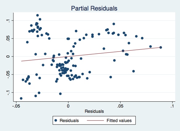
- Check whether there is a linear relationship between the residuals of the model (2.1) and the residuals of model (2.2). Draw your conclusion from what you see in the graph, and try to justify your answer in the light of basic assumptions of linear regression.
Please send comments to bottan2@illinois.edu or srmntbr2@illinois.edu?