Data Set

The data set used in this tutorial was borrowed from Johnston and DiNardo's Econometric Methods (1997, 4th ed), but slightly adjusted for your needs. It is called AUTO2. You can download the data by visiting the Econ 508 web site (Data). As you will see, this adapted data set contains five series.

    use AUTO2.dta, clear
    describe

  obs:           128                          AUTO2 adapted from Johnston and DiNardo, 1997
 vars:             5                          11 Sep 2002 12:22
 size:         2,560                          
-----------------------------------------------------------------------------------------------------
              storage  display     value
variable name   type   format      label      variable label
-----------------------------------------------------------------------------------------------------
quarter         float  %9.0g                  Quarter of the observation
gas             float  %9.0g                  Log of per capita real expenditure on gasoline and oil
price           float  %9.0g                  Log of the real price of gasoline and oil
income          float  %9.0g                  Log of per capita real disposable income
miles           float  %9.0g                  Log of miles per gallon
------------------------------------------------------------------------------------------------------
Sorted by:  

Summarizing the data

A useful recommendation for practitioners of Econometrics is to summarize the data set you are going to work with. This provides a "big picture” of the variables and what you can expect from them. You can do that by as follows:

    summarize    

    Variable |       Obs        Mean    Std. Dev.       Min        Max
-------------+--------------------------------------------------------
     quarter |       128     1974.75    9.270052     1959.1     1990.4
         gas |       128   -7.763027    .1201866  -8.019878  -7.606151
       price |       128    4.723974    .1658683   4.488154   5.176053
      income |       128    -4.19457     .153558   -4.50524  -3.969884
       miles |       128    2.712568    .1348134   2.583997   3.035914

Even better, you can ask for the details of each variable:

    summarize, detail

                  Quarter of the observation
-------------------------------------------------------------
      Percentiles      Smallest
 1%       1959.2         1959.1
 5%       1960.3         1959.2
10%       1962.1         1959.3       Obs                 128
25%      1966.75         1959.4       Sum of Wgt.         128

50%      1974.75                      Mean            1974.75
                        Largest       Std. Dev.      9.270052
75%      1982.75         1990.1
90%       1987.4         1990.2       Variance       85.93386
95%       1989.2         1990.3       Skewness       1.81e-17
99%       1990.3         1990.4       Kurtosis       1.798007

     Log of per capita real expenditure on gasoline and
                             oil
-------------------------------------------------------------
      Percentiles      Smallest
 1%    -8.016769      -8.019878
 5%    -8.005725      -8.016769
10%    -7.974048      -8.015248       Obs                 128
25%    -7.836869      -8.012581       Sum of Wgt.         128

50%    -7.719422                      Mean          -7.763027
                        Largest       Std. Dev.      .1201866
75%    -7.671802      -7.628435
90%     -7.64901      -7.625179       Variance       .0144448
95%    -7.636929      -7.620612       Skewness      -.9293219
99%    -7.620612      -7.606151       Kurtosis       2.503103

          Log of the real price of gasoline and oil
-------------------------------------------------------------
      Percentiles      Smallest
 1%     4.500299       4.488154
 5%     4.531126       4.500299
10%     4.557322       4.515703       Obs                 128
25%     4.621168        4.51949       Sum of Wgt.         128

50%     4.675815                      Mean           4.723974
                        Largest       Std. Dev.      .1658683
75%     4.767021       5.130968
90%     5.016708       5.149823       Variance       .0275123
95%     5.121161       5.162098       Skewness       1.180383
99%     5.162098       5.176053       Kurtosis       3.591608

          Log of per capita real disposable income
-------------------------------------------------------------
      Percentiles      Smallest
 1%    -4.498873       -4.50524
 5%    -4.490103      -4.498873
10%    -4.446543      -4.496271       Obs                 128
25%    -4.284298      -4.492739       Sum of Wgt.         128

50%    -4.158388                      Mean           -4.19457
                        Largest       Std. Dev.       .153558
75%    -4.105482      -3.978981
90%    -4.006467      -3.971754       Variance       .0235801
95%    -3.985354      -3.971611       Skewness        -.55278
99%    -3.971611      -3.969884       Kurtosis       2.312228

                   Log of miles per gallon
-------------------------------------------------------------
      Percentiles      Smallest
 1%     2.585882       2.583997
 5%     2.590767       2.585882
10%     2.596746       2.586259       Obs                 128
25%     2.613006       2.587764       Sum of Wgt.         128

50%      2.64715                      Mean           2.712568
                        Largest       Std. Dev.      .1348134
75%     2.812479       3.013695
90%     2.950735       3.021156       Variance       .0181746
95%     2.995482       3.028562       Skewness       1.069017
99%     3.028562       3.035914       Kurtosis        2.68393

Working with Time Series in Stata

The next step is to create the variables you will need to run dynamic models. Here you have two strategies:  
(i)  generate lags and differences using the command gen (explained in class)  
(ii)  convert your data set in time series, using the command tsset

Usually the strategy (ii) saves you time during the model selection process. Hence, following (ii), you need to generate a variable corresponding to the time period of each observation (which can not be “quarter” because it contains non-integer values):

    gen t = _n    
    label variable t "Integer time period"

Next you "tsset" your data using the created variable:

    tsset t

        time variable:  t, 1 to 128
                delta:  1 unit

Now you are ready to work with time series. The main operators you will need are:

1-period lag:	y(t-1)	type:	L.y
2-period lag:	y(t-2)	type:	L2.y
...
1-period lead:	y(t+1)	type:	F.y
2-period lead:	y(t+2)	type:	F2.y
...

Difference:	y(t) - y(t-1)	type:	D.y
Differerence of difference:	[y(t)-y(t-1)] - [y(t-1)-y(t-2)]	type:	D2.y
...
Seasonal difference:	y(t) - y(t-1)	type:	S.y
Lag-2 Seasonal difference	y(t) - y(t-1)	type:	S2.y
...

Graphing Time Series

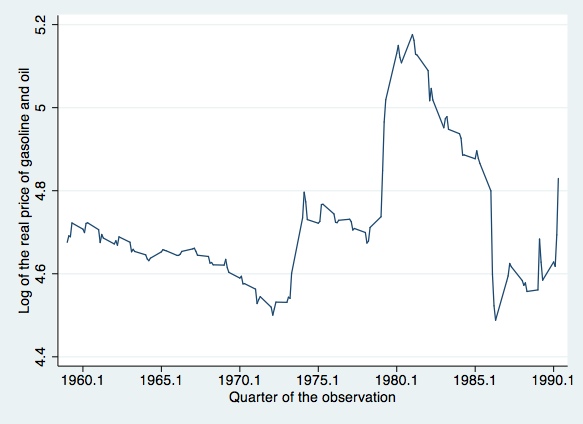
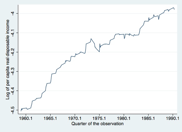
Next we will try to replicate some of Johnston and DiNardo's (1997, p. 267) graphical results

    line gas quarter, c(l) s(.) sort xlabel(1960.1 (5) 1990.1)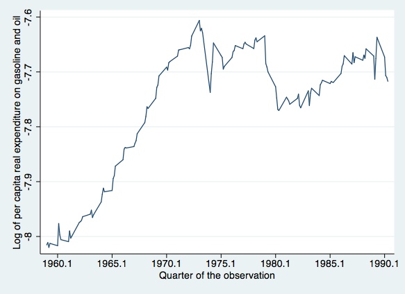

    line price quarter, c(l) s(.) sort xlabel(1960.1 (5) 1990.1)

  line income quarter, c(l) s(.) sort xlabel(1960.1 (5) 1990.1)

Running Dynamic Models

Next let’s run a typical dynamic model (Johnston and DiNardo, 1997, p. 269, Table 8.5):

    regress gas price L.price L2.price L3.price L4.price L5.price income L.income 
L2.income L3.income L4.income L5.income L.gas L2.gas L3.gas L4.gas L5.gas

      Source |       SS       df       MS              Number of obs =     123
-------------+------------------------------           F( 17,   105) =  383.71
       Model |  1.47998066    17  .087057686           Prob > F      =  0.0000
    Residual |  .023823131   105  .000226887           R-squared     =  0.9842
-------------+------------------------------           Adj R-squared =  0.9816
       Total |  1.50380379   122  .012326261           Root MSE      =  .01506

------------------------------------------------------------------------------
         gas |      Coef.   Std. Err.      t    P>|t|     [95% Conf. Interval]
-------------+----------------------------------------------------------------
       price |
         --. |  -.2676449   .0378744    -7.07   0.000    -.3427428    -.192547
         L1. |   .2628672   .0692914     3.79   0.000     .1254751    .4002592
         L2. |  -.0174063   .0754139    -0.23   0.818    -.1669381    .1321256
         L3. |  -.0720921   .0773891    -0.93   0.354    -.2255404    .0813562
         L4. |   .0143968   .0772103     0.19   0.852    -.1386968    .1674905
         L5. |   .0582077   .0463403     1.26   0.212    -.0336765    .1500919
             |
      income |
         --. |   .2927731   .1588226     1.84   0.068    -.0221427     .607689
         L1. |  -.1621984    .220227    -0.74   0.463    -.5988679    .2744712
         L2. |  -.0492554   .2143709    -0.23   0.819    -.4743133    .3758024
         L3. |   .0104172   .2131308     0.05   0.961    -.4121818    .4330161
         L4. |    .084901   .2101309     0.40   0.687    -.3317496    .5015517
         L5. |  -.1989616   .1531175    -1.30   0.197    -.5025654    .1046422
             |
         gas |
         L1. |   .6605733    .096063     6.88   0.000     .4700981    .8510485
         L2. |   .0670148   .1145346     0.59   0.560    -.1600861    .2941157
         L3. |  -.0235803   .1170941    -0.20   0.841    -.2557564    .2085957
         L4. |   .1321968    .119014     1.11   0.269     -.103786    .3681797
         L5. |   .1631249   .1013842     1.61   0.111    -.0379011     .364151
             |
       _cons |   .0055429   .1260436     0.04   0.965    -.2443782    .2554639
------------------------------------------------------------------------------

Long-run Elasticities

Suppose you wish to compute the long run income and price elasticities. Assuming that in the long-run the variables converge to their respective steady-state values (represented by "e”):

\[gas_{t}=gas_{t-1}=gas_{t-2}=...=gas_{e}\]
\[price_{t}=price_{t-1}=price_{t-2}=...=price_{e} \] \[income(t)=income(t-1)=income(t-2)=...=income_{e}, \]

and recalling that all variables are already in logs, you then just have to apply this steady state condition, reparameterize the model, and calculate the elasticities:

\[ \frac{d (gas(e))}{ d (income(e))}= \text{long run income elasticity} \] \[ \frac{d (gas(e))}{d (price(e))} = \text{long run price elasticity } \]

After that you can compare the long-run elasticities of the (reparameterized) dynamic model with the elasticities provided by the static version of this log-linear regression:

    regress gas price income

      Source |       SS       df       MS              Number of obs =     128
-------------+------------------------------           F(  2,   125) =  218.86
       Model |  1.42698222     2  .713491108           Prob > F      =  0.0000
    Residual |  .407508656   125  .003260069           R-squared     =  0.7779
-------------+------------------------------           Adj R-squared =  0.7743
       Total |  1.83449087   127   .01444481           Root MSE      =   .0571

------------------------------------------------------------------------------
         gas |      Coef.   Std. Err.      t    P>|t|     [95% Conf. Interval]
-------------+----------------------------------------------------------------
       price |  -.1502843   .0312311    -4.81   0.000    -.2120945   -.0884742
      income |   .7056134   .0337348    20.92   0.000     .6388481    .7723787
       _cons |  -4.093342   .2247555   -18.21   0.000    -4.538161   -3.648523
------------------------------------------------------------------------------

I suggest you to provide a little table comparing those results, and write your comments about how the elasticities differ from the static to the dynamic model.

In the light of the problem set, I suggest you to compute not only the point estimate of the elasticities, but also their confidence intervals. In the static model, confidence intervals are obtained directly from the regression output. But for the dynamic model, the elasticities are represented by a non-linear function of the parameters. In that case, you need to find confidence intervals for the elasticities using Delta-method or Bootstrap techniques, which you will see in professor Koenker's Lecture Note 5 and we will address in a future e-TA.

Impulse Response Functions

Here I recommend to use the best dynamic model (following the Schwarz Information Criterion that you will see in e-Tutorial 5), and to compute impulse response functions using the formula on Prof. Koenker's Lecture Note 3, page 3.

P.S.: Some authors propose alternative ways to calculate impulse response functions. One of them is to use partial derivatives (e.g., Enders, 1995, p.24), but such method has a drawback: it is quite easy to make a mistake when you have models with many lags and differences.

Usually it is expected that you account for a reasonable amount of response periods, depending on the structure of your data set. Usually we suggest a minimum of 40 (forty) response periods for quarterly data. Then you plot those responses along the respective time scale (t=0,1,2,3,...,40). This will generate the non-cumulative impulse response function. If you wish a cumulative impulse response function, at each new period t+i (i=1,2,3,...), you should add the effect to the previous shocks.