e-TA 2: Box-Cox and Partial Residual Plot
Welcome to e-Tutorial, your on-line help to Econ508. The present issue focuses on the basic operations of R. The introductory material presented below is designed to enhance your understanding of the topics and your performance on the homework. This issue focuses on the basic features of Box-Cox transformations and Partial Residual Plots.1
Introduction
In problem set 1, question 1, you are asked to estimate two demand equations for bread using the data set available here (or if you prefer, visit the data set collection at the Econ 508 web page, under the name "giffen"). You can save the data using the techniques suggested on e-Tutorial 1. As a general guideline, I suggest you to script your work.
Parts (i)-(iii) of the problem set involve simple linear regression and hypothesis testing that should be straightforward to solve once you are familiar with Stata. For every hypothesis testing, please make clear what are the null and alternative hypotheses. Please also provide a simple table with the main estimation results. I recommend you to ALWAYS include standard deviations for ALL parameters you estimate. Remember the first rule of empirical paper writing: "All good estimates deserve a standard error". Another useful advice is to summarize your main conclusions. It is strongly encouraged that you structure your problem set as a paper. Finally, graphs are very welcome as long as you provide labels and refer to them on your comments. Don't include any remaining material (e.g., software output or your preliminary regressions) in your report.
Partial Residual Plot
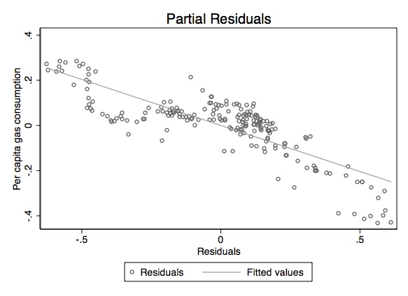
Question 1, part (iv) requires you to compare the plots of the Engel curves for bread in the "short" and "long" versions of the model using partial residual plot for the latter model. As mentioned in Professor Koenker's Lecture 2, "the partial residual plot is a device for representing the final step of a multivariate regression result as a bivariate scatterplot." Here is how you do that:
Theorem: (Gauss-Frisch-Waugh)
Recall the results of the Gauss-Frisch-Waugh theorem in Professor Koenker's Lecture Note 2 (pages 8-9). Here you will see that you can obtain the same coefficient and standard deviation for a given covariate by using partial residual regression. I will show the result using the gasoline demand data available here. In this data set, Y corresponds to the log per capita gas consumption, P is the log gas price, and Z is the log per capita income. The variables are already in the logarithmic form, so that we are actually estimating log-linear models.
At first you run the full model (Model A) and observe the
coefficient and standard deviation of P. Then you run a shorter version
of the model (Model B), excluding P. You get the residuals of this
partial regression and call them "resB". After that you run another
short model (Model C), but in this case you regress the omitted
variable P on the same covariates of model B. You obtain the residuals
of the latter model and call them "resC". Finally, you regress the
residuals of the model B on the residuals of the model C.
    insheet using gasnew.dat, clear
    describe
Contains data
obs: 201
vars: 4
size: 3,216
--------------------------------------------------------------
storage display value
variable name type format label variable label
--------------------------------------------------------------
year float %9.0g
lnp float %9.0g ln(p)
lnz float %9.0g ln(z)
lny float %9.0g ln(y)
--------------------------------------------------------------
Sorted by:
Note: dataset has changed since last saved
gen Y=lny
genP=lnp
genZ=lnz
* Model A: Y = \alpha_{0} + \alpha_{1}*P + \alpha_{2}*Z
regress Y P Z
* Model B: Y = \beta_{0} + \beta_{1}*Z
regressY Z
* Residual Model B
predict resB, resid
* Model C: P = \gamma_{0} + \gamma_{1}*Z
regressP Z
* Residual Model C
predictresC, resid
* Gauss-Frisch-Waugh: resB = \theta_{0} + \theta_{1}*resC
regressresB resC
. * Model A: Y = \alpha_{0} + \alpha_{1}*P + \alpha_{2}*Z

.     regress Y P Z

      Source |       SS       df       MS              Number of obs =     201
-------------+------------------------------           F(  2,   198) = 1674.11
       Model |  21.0866833     2  10.5433417           Prob > F      =  0.0000
    Residual |  1.24698236   198  .006297891           R-squared     =  0.9442
-------------+------------------------------           Adj R-squared =  0.9436
       Total |  22.3336657   200  .111668328           Root MSE      =  .07936

------------------------------------------------------------------------------
           Y |      Coef.   Std. Err.      t    P>|t|     [95% Conf. Interval]
-------------+----------------------------------------------------------------
           P |  -.4075322   .0196435   -20.75   0.000    -.4462696   -.3687948
           Z |    1.75935   .0419446    41.94   0.000     1.676634    1.842065
       _cons |  -5.266504   .1121704   -46.95   0.000    -5.487706   -5.045303
------------------------------------------------------------------------------

. * Model B: Y = \beta_{0} + \beta_{1}*Z

.     regress Y Z

      Source |       SS       df       MS              Number of obs =     201
-------------+------------------------------           F(  1,   199) =  923.98
       Model |  18.3759978     1  18.3759978           Prob > F      =  0.0000
    Residual |  3.95766793   199  .019887779           R-squared     =  0.8228
-------------+------------------------------           Adj R-squared =  0.8219
       Total |  22.3336657   200  .111668328           Root MSE      =  .14102

------------------------------------------------------------------------------
           Y |      Coef.   Std. Err.      t    P>|t|     [95% Conf. Interval]
-------------+----------------------------------------------------------------
           Z |   .9735875   .0320289    30.40   0.000     .9104278    1.036747
       _cons |  -3.106386   .0741504   -41.89   0.000    -3.252608   -2.960165
------------------------------------------------------------------------------

. * Residual Model B

.     predict resB, resid

. * Model C: P = \gamma_{0} + \gamma_{1}*Z

.     regress P Z

      Source |       SS       df       MS              Number of obs =     201
-------------+------------------------------           F(  1,   199) =  878.73
       Model |  72.0708177     1  72.0708177           Prob > F      =  0.0000
    Residual |   16.321319   199  .082016678           R-squared     =  0.8154
-------------+------------------------------           Adj R-squared =  0.8144
       Total |  88.3921367   200  .441960684           Root MSE      =  .28639

------------------------------------------------------------------------------
           P |      Coef.   Std. Err.      t    P>|t|     [95% Conf. Interval]
-------------+----------------------------------------------------------------
           Z |   1.928099    .065043    29.64   0.000     1.799837    2.056361
       _cons |  -5.300484   .1505815   -35.20   0.000    -5.597424   -5.003544
------------------------------------------------------------------------------

. * Residual Model C

.     predict resC, resid

. * Gauss-Frisch-Waugh: resB = \theta_{0} + \theta_{1}*resC

.     regress resB resC

      Source |       SS       df       MS              Number of obs =     201
-------------+------------------------------           F(  1,   199) =  432.59
       Model |  2.71068559     1  2.71068559           Prob > F      =  0.0000
    Residual |  1.24698237   199  .006266243           R-squared     =  0.6849
-------------+------------------------------           Adj R-squared =  0.6833
       Total |  3.95766796   200   .01978834           Root MSE      =  .07916

------------------------------------------------------------------------------
        resB |      Coef.   Std. Err.      t    P>|t|     [95% Conf. Interval]
-------------+----------------------------------------------------------------
        resC |  -.4075322   .0195941   -20.80   0.000     -.446171   -.3688934
       _cons |  -5.37e-10   .0055835    -0.00   1.000    -.0110104    .0110104
------------------------------------------------------------------------------
Next we can plot those residuals and insert a fitting line:
   graph twoway (scatter resB resC, m(oh)) (lfit resB resC), sch(s1mono)
 ytitle(Per capita gas consumption) title(Partial Residuals)
Box-Cox Transformation:
For question 2, parts (a)-(d) are also straightforward. You are expected to calculate the estimates in both linear and log-linear form. Besides them, you are expected to run a Box-Cox version of the model, and interpret it. Here I will give you some help by using the same gasoline demand data as above.
Just for a minute, suppose somebody told you that a nice gasoline demand equation should also include two additional covariates: the squared price of gas, and the effect of price times income. You can obtain those variables as follows:
gen Psq = P^2
genPZ = P*Z
Next you are asked to run this extended model, in a traditional log-linear form (remember that all covariates are already in logs). So, the easiest way to do that is as follows:
regress Y P Z Psq PZ
      Source |       SS       df       MS              Number of obs =     201
-------------+------------------------------           F(  4,   196) = 1499.50
       Model |  21.6269476     4   5.4067369           Prob > F      =  0.0000
    Residual |  .706718113   196  .003605705           R-squared     =  0.9684
-------------+------------------------------           Adj R-squared =  0.9677
       Total |  22.3336657   200  .111668328           Root MSE      =  .06005

------------------------------------------------------------------------------
           Y |      Coef.   Std. Err.      t    P>|t|     [95% Conf. Interval]
-------------+----------------------------------------------------------------
           P |  -2.573682   .1858084   -13.85   0.000    -2.940122   -2.207242
           Z |   2.571179    .077643    33.12   0.000     2.418056    2.724302
         Psq |  -.2712707   .0375378    -7.23   0.000    -.3453005   -.1972408
          PZ |   .7170179   .0593085    12.09   0.000     .6000532    .8339826
       _cons |  -7.391471   .2032132   -36.37   0.000    -7.792236   -6.990706
------------------------------------------------------------------------------
The log-linear form seems to be a nice attempt to estimate the gasoline demand.
Next, suppose you are so confident on this model that you write a paper about the topic and send it to a journal. Two weeks later you receive a letter from a referee saying she is suspicious about your log-linear equation. She asks you to reestimate the same model but using the dependent variable linearly (i.e., without the logs), and the rest of the equation remaining as before. She asks you to revise and resubmit the paper with your new findings.
In the search for elements that support your original model, you start the following experiment: 1. Run the model suggested by the referee, using a Box-Cox transformation to find the MLE ofλ, 2. Plot the concentrated log-likelihood function, and 3. Reestimate the model conditional on the MLE of λ:
geny = exp(Y)
boxcox y P Z Psq PZ, level(95)
Fitting comparison model

Iteration 0:   log likelihood =  110.10193
Iteration 1:   log likelihood =  112.76717
Iteration 2:   log likelihood =  112.77299
Iteration 3:   log likelihood =  112.77299

Fitting full model

Iteration 0:   log likelihood =  426.09821
Iteration 1:   log likelihood =  458.18797
Iteration 2:   log likelihood =  458.18823
Iteration 3:   log likelihood =  458.18823

                                                  Number of obs   =        201
                                                  LR chi2(4)      =     690.83
Log likelihood = 458.18823                        Prob > chi2     =      0.000

------------------------------------------------------------------------------
           y |      Coef.   Std. Err.      z    P>|z|     [95% Conf. Interval]
-------------+----------------------------------------------------------------
      /theta |   -.050263   .1154772    -0.44   0.663    -.2765942    .1760682
------------------------------------------------------------------------------

Estimates of scale-variant parameters
----------------------------
             |      Coef.
-------------+--------------
Notrans      |
           P |  -2.624961
           Z |   2.658853
         Psq |  -.2801617
          PZ |   .7253629
       _cons |  -7.633947
-------------+--------------
      /sigma |   .0619262
----------------------------

---------------------------------------------------------
   Test         Restricted     LR statistic      P-value
    H0:       log likelihood       chi2       Prob > chi2
---------------------------------------------------------
theta = -1       423.34476        69.69           0.000
theta =  0       458.09427         0.19           0.665
theta =  1       426.09821        64.18           0.000
---------------------------------------------------------
version 6: boxcox y P Z Psq PZ, level(95) graph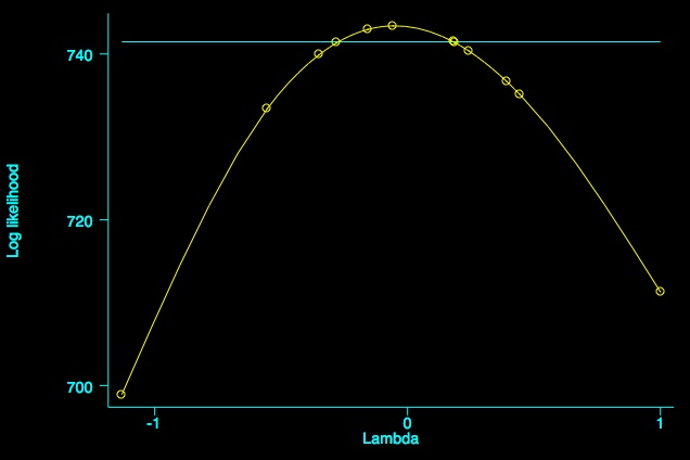
As you see, the MLE for λ is very close to zero (-0.050263). The picture is drawn using smoothing spline techniques to help you envisage the log-likelihood function and the MLE of λ. The horizontal line corresponds to the 95% confidence interval. Next we can apply the power transform to y and then fit the revised model:
qui:boxcox y P Z Psq PZ, level(95)
gen ytrans=((y^r(est))-1)/r(est)
regressytrans P Z Psq PZ
      Source |       SS       df       MS              Number of obs =     201
-------------+------------------------------           F(  4,   196) = 1507.45
       Model |  23.7132269     4  5.92830673           Prob > F      =  0.0000
    Residual |  .770805496   196  .003932681           R-squared     =  0.9685
-------------+------------------------------           Adj R-squared =  0.9679
       Total |  24.4840324   200  .122420162           Root MSE      =  .06271

------------------------------------------------------------------------------
      ytrans |      Coef.   Std. Err.      t    P>|t|     [95% Conf. Interval]
-------------+----------------------------------------------------------------
           P |  -2.624961   .1940504   -13.53   0.000    -3.007656   -2.242266
           Z |   2.658853   .0810871    32.79   0.000     2.498938    2.818768
         Psq |  -.2801617   .0392029    -7.15   0.000    -.3574754    -.202848
          PZ |   .7253629   .0619393    11.71   0.000     .6032099    .8475158
       _cons |  -7.633947   .2122272   -35.97   0.000    -8.052489   -7.215405
------------------------------------------------------------------------------
The latter regression (conditional on the MLE of λ) provides results
close to your log-linear suggestion. Now you have reasonable support to
write back the referee and defend your original model.
Andrews Test
Finally, for the Econ 508 problem set 1, question 2, you are also required to perform the David Andrews (1971) test. As an example, I use the same gasoline data as above, and follow the routine on Professor Koenker's Lecture Note 2:
- Run the linear model and get the predicted values of y (call this variable \(\hat y\)):
genp=exp(P)gen
z=exp(Z)regress
y p z
      Source |       SS       df       MS              Number of obs =     201
-------------+------------------------------           F(  2,   198) = 1609.94
       Model |  3.70695117     2  1.85347559           Prob > F      =  0.0000
    Residual |  .227951976   198  .001151273           R-squared     =  0.9421
-------------+------------------------------           Adj R-squared =  0.9415
       Total |  3.93490315   200  .019674516           Root MSE      =  .03393

------------------------------------------------------------------------------
           y |      Coef.   Std. Err.      t    P>|t|     [95% Conf. Interval]
-------------+----------------------------------------------------------------
           p |  -.3375906   .0144982   -23.28   0.000    -.3661814   -.3089999
           z |   .0741067   .0016292    45.49   0.000     .0708939    .0773195
       _cons |  -.1536729   .0112284   -13.69   0.000    -.1758155   -.1315303
------------------------------------------------------------------------------
predict yhat- Reestimate the augmented model and test (\gamma = 0):
genLY=log(yhat)
genYLY=yhat*LY
regressy p z YLY
      Source |       SS       df       MS              Number of obs =     201
-------------+------------------------------           F(  3,   197) = 1610.62
       Model |  3.78075786     3  1.26025262           Prob > F      =  0.0000
    Residual |   .15414529   197  .000782463           R-squared     =  0.9608
-------------+------------------------------           Adj R-squared =  0.9602
       Total |  3.93490315   200  .019674516           Root MSE      =  .02797

------------------------------------------------------------------------------
           y |      Coef.   Std. Err.      t    P>|t|     [95% Conf. Interval]
-------------+----------------------------------------------------------------
           p |  -.2958436   .0127019   -23.29   0.000    -.3208928   -.2707945
           z |   .0651617   .0016286    40.01   0.000     .0619501    .0683734
         YLY |   1.082626   .1114711     9.71   0.000     .8627956    1.302455
       _cons |   .2845145   .0460572     6.18   0.000     .1936861     .375343
------------------------------------------------------------------------------
test YLY
 ( 1)  YLY = 0

       F(  1,   197) =   94.33
            Prob > F =    0.0000
From the test above we can reject the null hypothesis that (\gamma =0). Can you interpret what does this mean?
Please send comments to bottan2@illinois.edu or srmntbr2@illinois.edu