e-TA 1: Brief Introduction to Stata
Welcome to e-Tutorial, your on-line help to Econ508. The introductory material presented below is the first of a series of handouts that will be distributed along the course, designed to enhance your understanding of the topics and your performance on the homework. This very first issue focuses on the basic operations of the main software used in the course (STATA). The core material was extracted from Gregory Kordas' "Computing in Econ 472" (1999) and "A Tutorial in Stata" (1999). The usual disclaimers apply.1
Accessing Stata
The statistical package Stata can be found at the OCSS (Office of
Computing and Communications for Social Sciences) lab, located at the
212 Lincoln Hall. Also, you can find Stata at the Foreign Languages
Building (FLB) (room G8). It is also available at the Econometrics Lab,
DKH, for students enrolled in the Econometrics field or other classes
that require lab experiments.Stata is probably the most widely used statstical software for applied econometrics. It already comes with an extensive library of functions and it is possible to easily download user-written functions. Additionally, Stata has an extraordinary set of reference books, and by this reason some students may be interested in purchasing the package. In those cases, the best strategy is to form a group of students and make a special order to STATA Inc. For Econ 508 purposes, however, the weekly edition of e-Tutorial will bring all necessary information to solve the homework. A very important resource to keep in mind whenever you encounter a problem not descibed in the manuals is the official Stata forums at statalist.org
First steps in Stata
Having installed Stata the next step is learning the syntax of the language, this means learning the rules of it. After you open Stata you are going to see the Stata console, which displays the results of your analysis or any messages associated with your code that is entered in the command line (the box at the bottom of the screen).
For example, we can use Stata as a calculator. In the command box you can type:
display 2 + 2 4or
displaylog(1)
0To quit the program just type:
exit, clearNote: most Stata commands have several options options which are invoked after placing the ",". In the example above, if data were loaded in the memory then typing "exit" only would give the following error:
 no; data in memory would be lost
r(4);
therefore, it is necessary to clear the data from the memory before exiting Stata.
This could be done in two lines of command by typing "clear" first and
then "exit". Or by using the clear option of the "exit" command (as
above). To learn more about what a command does and its options, you
can always refer to its help file by typing:
help exitScripting your work
Rather than saving the work space, it is highly recommended that you
keep a record of the commands entered, so that we can reproduce it at a
later date. The easiest way to do this is to record all your commands
on a do-file,
available from the File menu. Commands are executed by highlighting
them and hitting Run (or Ctrl+Shift+D for PC and Command+Shift+D for
Mac). At the end of a session, save the final script for a permanent
record of your work.
A do-file is a text file that contains lines of Stata code that can be saved and use over and over again. This is the preferred method to save your work and guarantee reproducibility. To know more on reproducible research you should read Professor Koenker's Reproducibility in Econometrics Research webpage
A useful tip to keep in mind is that everything that is written
after a * sign is assumed to be a comment and is ignored by Stata.
Working in Stata
The best way to learn Stata is to dive right in and work through a simple example.
Example - The U.S. Economy in the 1990s
Let's start with an analysis of the performance of the U.S. economy during the 1990s. We have annual data on GDP growth, GDP per capita growth, private consumption growth, investment growth, manufacturing labor productivity growth, unemployment rate, and inflation rate. (The data is publicly available in the statistical appendixes of the World Economic Outlook, May 2001, IMF).
The first step is to tell Stata the location of your working
directory. This means telling Stata where are all the files related to
your project. You should do this always at the beginning of your
session. You do so by using the cd path function. Where path is the path to the folder where you want to write and read things. For example
cd "C:\Econ508\eTA\"This command line is telling Stata to read and write everything in
the Econ508\eTA folder (that I assume you created before hand).The next step is to download the data. The data is available in in text format here. To load the data, type:
insheet using "US90.txt"In the commands above, the term insheet refers to the action executed by Stata, this is followed by using after which we must indicate the name of the file we want to load. insheet
can be used when the data is delimited and Stata will automatically
detect the type of delimiting used (i.e. comma-separated, tabs, etc.).
For ASCII data with *.raw format, you must use the infile command.
After that you can visualize the data in a spread-sheet format type browse. Or to visualize small data sets you can also type:
list +-------------------------------------------------------------------+
| year gdpgr consgr invgr unemp gdpcapgr inf producgr |
|-------------------------------------------------------------------|
1. | 1992 3.1 2.9 5.2 7.5 1.9 3 5.1 |
2. | 1993 2.7 3.4 5.7 6.9 1.5 3 1.9 |
3. | 1994 4 3.8 7.3 6.1 3 2.6 3 |
4. | 1995 2.7 3 5.4 5.6 1.7 2.8 3.9 |
5. | 1996 3.6 3.2 8.4 5.4 2.6 2.9 3.4 |
|-------------------------------------------------------------------|
6. | 1997 4.4 3.6 8.8 5 3.4 2.3 3.8 |
7. | 1998 4.4 4.7 10.7 4.5 3.4 1.5 6.2 |
8. | 1999 4.2 5.3 9.1 4.2 3.2 2.2 5.8 |
9. | 2000 5 5.3 8.8 4 4.2 3.4 7.2 |
10. | 2001 1.5 2.5 3.3 4.4 .7 2.6 4.1 |
|-------------------------------------------------------------------|
11. | 2002 2.5 2.4 3.8 5 1.8 2.2 3 |
+-------------------------------------------------------------------+
count 11 save US90file US90.dta savedBasic Operations
A useful way to explore your data is checking the main statistics of each variable. For example, in the Stata Command window you can obtain the minimum, maximum, arithmetic mean, and standard deviation of each variable in your data set by typing:
summarize
    Variable |       Obs        Mean    Std. Dev.       Min        Max
-------------+--------------------------------------------------------
        year |        11        1997    3.316625       1992       2002
       gdpgr |        11    3.463636    1.050974        1.5          5
      consgr |        11    3.645455     1.03476        2.4        5.3
       invgr |        11    6.954545    2.408885        3.3       10.7
       unemp |        11    5.327273    1.125247          4        7.5
-------------+--------------------------------------------------------
    gdpcapgr |        11    2.490909    1.048289         .7        4.2
         inf |        11    2.590909    .5204893        1.5        3.4
    producgr |        11    4.309091    1.590883        1.9        7.2
If you are only interested in a single variable, just include its name after the command:
summarizegdpgr
    Variable |       Obs        Mean    Std. Dev.       Min        Max
-------------+--------------------------------------------------------
       gdpgr |        11    3.463636    1.050974        1.5          5
If you also wish to know the behavior along the percentiles for the variable gdpgr, type
summarizegdpgr, detail
                            gdpgr
-------------------------------------------------------------
      Percentiles      Smallest
 1%          1.5            1.5
 5%          1.5            2.5
10%          2.5            2.7       Obs                  11
25%          2.7            2.7       Sum of Wgt.          11

50%          3.6                      Mean           3.463636
                        Largest       Std. Dev.      1.050974
75%          4.4            4.2
90%          4.4            4.4       Variance       1.104545
95%            5            4.4       Skewness      -.3234939
99%            5              5       Kurtosis       2.156121
If you are only interested in a subset of your data, you can inspect
it using filters. E.g., if you are only interested gdp growth in the
years of the Clinton administration, you type
summarizegdpgr if year>=1993 & year<=2000
    Variable |       Obs        Mean    Std. Dev.       Min        Max
-------------+--------------------------------------------------------
       gdpgr |         8       3.875    .8259194        2.7          5
And then you can contrast that period with the family Bush administrations:
summarizegdpgr if year<1993 | year>2000
    Variable |       Obs        Mean    Std. Dev.       Min        Max
-------------+--------------------------------------------------------
       gdpgr |         3    2.366667    .8082903        1.5        3.1
You may also check all years but the election years, to avoid political cycles:
summarizegdpgr if year~= 2000 & year~=1996 & year~=1992
    Variable |       Obs        Mean    Std. Dev.       Min        Max
-------------+--------------------------------------------------------
       gdpgr |         8         3.3    1.090216        1.5        4.4
At this point you have already noticed the main logical operators in Stata:
>= means "greater or equal",
<= means "less or equal",
& means "and",
| means "or".
The arithmetic operators are as usual (+, -, *, /). And to create a
new variable using them, you can do as follows: Suppose you wish to
know how close the GDP growth is to the GDP per capita growth. So, you
create a ratio of those two variables, and check it:
generategdpratio = gdpgr / gdpcapgr
summarize gdpratio
    Variable |       Obs        Mean    Std. Dev.       Min        Max
-------------+--------------------------------------------------------
    gdpratio |        11    1.487338    .2820946   1.190476   2.142857
The same procedure can be done to obtain traditional transformations, such as
squares: gen produc2=producgr^2
square roots: gen infroot=sqrt(inf)
exponential: gen expgdpgr=exp(gdpgr)
natural logs: gen logunemp=log(unemp) or simply gen lnunemp=ln(unemp)
base 10 logs: gen log10inf=log10(inf)
A final remark is that you should choose a name for the generated
variable with at most 32 characters (or less depending on the version
of Stata you are using), otherwise the system will give an error
message. Nevertheless, you can always (and maybe should for
convenience) describe your variables in more detail using the commands label or notes.
Exploring Graphical Resources
Suppose now you want to check the relationship among variables. For example, you want to see how much consumption and investment are correlated with GDP (all variables in growth rates). The command for that is:
graph twoway (scatter gdpgr year)(scatterconsgr year)(scatterinvgr year)
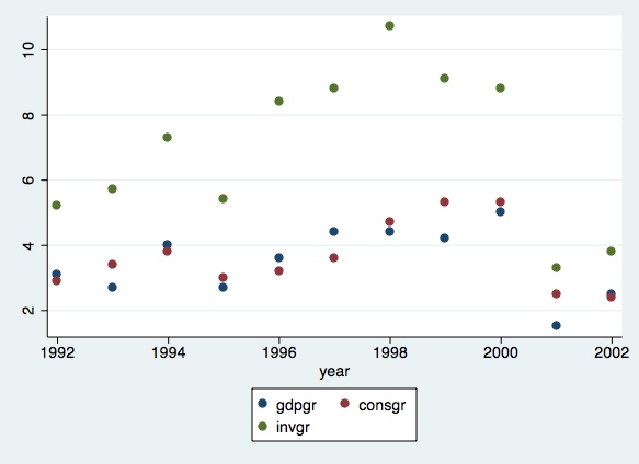
The output is a scatter of points for each series, with the
investment series being relatively higher than the other two series. If
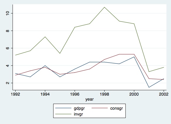
you are interested in a line graph. The command is as follows:
graph twoway (line gdpgr year)(lineconsgr year)(lineinvgr year)
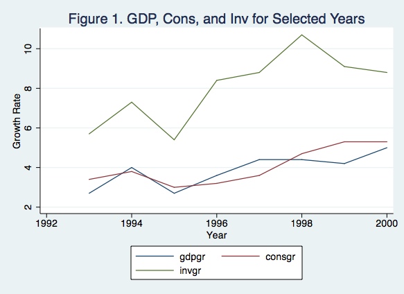
To plot specific ranges, add a title and name the axis:
graph twoway (line gdpgr year if year>=1993 & year<=2000)(lineconsgr year if
year>=1993 & year<=2000)(lineinvgr year if year>=1993 & year<=2000), title("Figure 1.
GDP, Cons, and Inv for Selected Years") xtitle("Year") ytitle("Growth Rate")
Finally, you can combine graphs in a single figure. For example,
suppose you would like to obtain a graphical diagnostic on the
relationship between GDP and consumption growth rates, GDP and
investment growth rates, GDP and productivity growth rates, and revisit
the relation between unemployment and inflation rates. The commands to
do that are as follows:
scatter gdpgr consgr, saving(part1)scattergdpgr invgr, saving(part2)scattergdpgr producgr, saving(part3)scatterunemp inf, saving(part4)
graph combine part1.gph part2.gph part3.gph part4.gph
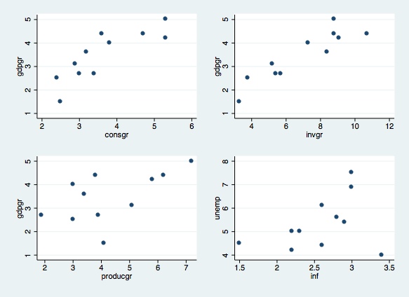
Through the commands above, you generated and saved four individual
graphs, and plotted them into a single figure. This is indeed a
very useful tool to check pair wise correlation among variables, before
you run a regression.
Linear Regression
As remarked above, before running a regression, it is recommended to check the cross correlation among covariates. You can do that graphically (see above) or using the following simple command:
correlate gdpgr consgr invgr unemp gdpcapgr inf | gdpgr consgr invgr unemp gdpcapgr inf
-------------+---------------------------------------------------------------
gdpgr | 1.0000
consgr | 0.8394 1.0000
invgr | 0.9097 0.8270 1.0000
unemp | -0.3035 -0.4761 -0.3684 1.0000
gdpcapgr | 0.9890 0.8347 0.8841 -0.4143 1.0000
inf | -0.1012 -0.1198 -0.3090 0.3590 -0.1230 1.0000
From the matrix above you can see, for example, that GDP and GDP per capita growth rates are closely related, but each of them has a different degree of connection with unemployment rates (in fact, GDP per capita presents higher correlation with unemployment rates than total GDP). Inflation and unemployment present a reasonable degree of positive correlation (about 36%).
Now you start with simple linear regressions. For example, let's
check the individual regressions of GDP with consumption and investment
growth rates:
regress gdpgr consgr
      Source |       SS       df       MS              Number of obs =      11
-------------+------------------------------           F(  1,     9) =   21.46
       Model |  7.78197201     1  7.78197201           Prob > F      =  0.0012
    Residual |  3.26348251     9  .362609168           R-squared     =  0.7045
-------------+------------------------------           Adj R-squared =  0.6717
       Total |  11.0454545    10  1.10454545           Root MSE      =  .60217

------------------------------------------------------------------------------
       gdpgr |      Coef.   Std. Err.      t    P>|t|     [95% Conf. Interval]
-------------+----------------------------------------------------------------
      consgr |   .8525216   .1840263     4.63   0.001     .4362251    1.268818
       _cons |   .3558076   .6949943     0.51   0.621    -1.216379    1.927994
------------------------------------------------------------------------------
regress gdpgr invgr
      Source |       SS       df       MS              Number of obs =      11
-------------+------------------------------           F(  1,     9) =   43.22
       Model |  9.14164404     1  9.14164404           Prob > F      =  0.0001
    Residual |  1.90381048     9  .211534498           R-squared     =  0.8276
-------------+------------------------------           Adj R-squared =  0.8085
       Total |  11.0454545    10  1.10454545           Root MSE      =  .45993

------------------------------------------------------------------------------
       gdpgr |      Coef.   Std. Err.      t    P>|t|     [95% Conf. Interval]
-------------+----------------------------------------------------------------
       invgr |   .3969137   .0603774     6.57   0.000     .2603305    .5334969
       _cons |   .7032821   .4422039     1.59   0.146    -.2970526    1.703617
------------------------------------------------------------------------------
Please note that you don't need to include the intercept, because
STATA automatically includes it. In the output above you have the main
regression diagnostics (ANOVA, adjusted R-squared, t-statistics, sample
size, etc.). The same rule apply to multiple linear regressions. For
example, suppose you want to find the main sources of GDP growth. You
type:
regress gdpgr consgr invgr producgr unemp inf
      Source |       SS       df       MS              Number of obs =      11
-------------+------------------------------           F(  5,     5) =    7.27
       Model |  9.70924721     5  1.94184944           Prob > F      =  0.0242
    Residual |  1.33620731     5  .267241462           R-squared     =  0.8790
-------------+------------------------------           Adj R-squared =  0.7581
       Total |  11.0454545    10  1.10454545           Root MSE      =  .51695

------------------------------------------------------------------------------
       gdpgr |      Coef.   Std. Err.      t    P>|t|     [95% Conf. Interval]
-------------+----------------------------------------------------------------
      consgr |   .1822094   .3605194     0.51   0.635    -.7445351    1.108954
       invgr |   .3448859   .1338048     2.58   0.050     .0009296    .6888422
    producgr |   .0490201   .1547288     0.32   0.764    -.3487228    .4467631
       unemp |   .0551669   .1897954     0.29   0.783    -.4327176    .5430514
         inf |   .3019558    .372596     0.81   0.455    -.6558326    1.259744
       _cons |  -.8865854   1.492931    -0.59   0.578    -4.724287    2.951116
------------------------------------------------------------------------------
In the example above, despite we have a high adjusted R-squared, most of the covariates are not significant at 5% level (actually, only the investments coefficient is significant at this level). There may be many problems in the regression above. On the Econ 508 classes you will learn how to solve most of those problems, including how to select the best specification for a model.
You can also run a log-linear regression after transforming each variable into a natural log scale. To do so, you type:gen lngdpgr=ln(gdpgr)
gen lnconsgr=ln(consgr)
gen lninvgr=ln(invgr)
gen lnproduc=ln(producgr)
gen lnunemp=ln(unemp)
gen lninf=ln(inf)
regress lngdpgr lnconsgr lninvgr lnproduc lnunemp lninf
      Source |       SS       df       MS              Number of obs =      11
-------------+------------------------------           F(  5,     5) =    7.19
       Model |  1.07467131     5  .214934262           Prob > F      =  0.0247
    Residual |  .149400242     5  .029880048           R-squared     =  0.8779
-------------+------------------------------           Adj R-squared =  0.7559
       Total |  1.22407155    10  .122407155           Root MSE      =  .17286

------------------------------------------------------------------------------
     lngdpgr |      Coef.   Std. Err.      t    P>|t|     [95% Conf. Interval]
-------------+----------------------------------------------------------------
    lnconsgr |    .114882   .4666926     0.25   0.815     -1.08479    1.314554
     lninvgr |    .779761   .3081229     2.53   0.052    -.0122942    1.571816
    lnproduc |   .0950277   .1935535     0.49   0.644    -.4025174    .5925728
     lnunemp |   .2009322   .3716735     0.54   0.612    -.7544849    1.156349
       lninf |   .1184624   .2785439     0.43   0.688    -.5975574    .8344822
       _cons |  -.9912522    .787582    -1.26   0.264    -3.015796    1.033292
------------------------------------------------------------------------------
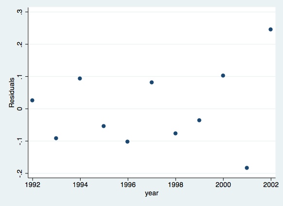
Finally, you can generate predicted values of the dependent variable and of the residuals, and plot them:
predict lngdpfitscatterlngdpfit year
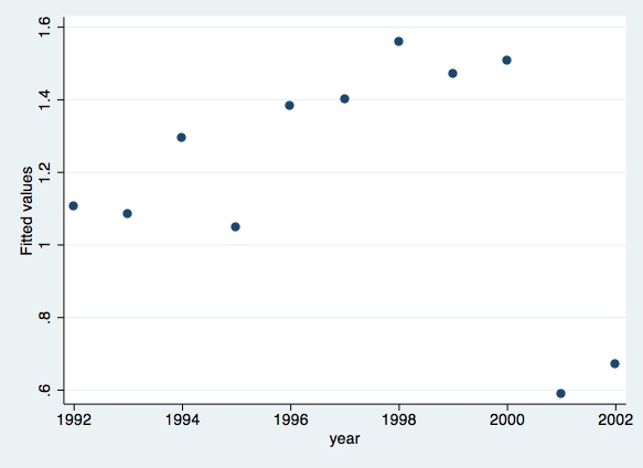
predict lngdpres, residscatterlngdpresyear
Linear Hypothesis Testing
After running the regressions above, we can proceed with tests of
linear hypothesis on the covariates. For example, suppose you would
like to be sure that investment growth "matters" to GDP growth.
Thus, you proceed with:
test lninvgr ( 1) lninvgr = 0
F( 1, 5) = 6.40
Prob > F = 0.0525 You just performed a F-test for the null hypothesis of lninvgr=0 against the alternative of lninvgr ~= 0. The computed F-statistic is the squared of the popular t-statistic. The result means that investment growth rates (in logs) are significantly different than zero at 5.25% level, and therefore they contribute to explain the variation in GDP growth rates (in logs).
To test the joint significance of two or more covariates, you type:
test lninvgr lnconsgr lnproduc ( 1) lninvgr = 0
( 2) lnconsgr = 0
( 3) lnproduc = 0
F( 3, 5) = 11.40
Prob > F = 0.0113
Here you are testing the null hypothesis that all covariates are zero against the alternative hypothesis that at least one of them is different than zero. The result shows that we cannot accept the null at 1.13% of significance, i.e., some of them are significantly different than zero at this level. So, some of them "matter" in explaining the variation in GDP growth rates (logs) along the years.
You could also extend your tests and check the equality of
covariates. For example, suppose you would like to know if investments
and consumption have similar coefficients:
test lninvgr=lnconsgr( 1) - lnconsgr + lninvgr = 0
F( 1, 5) = 0.79
Prob > F = 0.4143
This is similar to test whether their difference is zero (null
hypothesis) or different than zero (alternative). The conclusion is
that, at 5% significance level, we cannot reject the null hypothesis of
similarity.
Please send comments to bottan2@illinois.edu or srmntbr2@illinois.edu