
e-TA 17: Survival Analysis
Welcome to a new issue of e-Tutorial. This e-TA will focus on on Duration Models (a.k.a. Survival Analysis) in the context of the PS5. 1
Data
You can download the data set, called weco14.csv from the Econ 508 web site. Save it in your preferred directory.
See the first section of e-TA 13 on Cubic B-Splines and Quantile Regression for description on preparing the data and saving it in Stata format.
use weco14.dta, clearNext generate the variables needed:
gen lex2 = lex^2Survival Analysis
Kaplan-Meier
In Stata, the first thing you need to do is to declare your data set as a survival-time data. You need to identify the "analysis time" variable, and the "failure" variable. The former indicates the duration of the process, while the latter indicates whether the data is censored. In the PS5 data set, "job_tenure" represents the "analysis-time" variable, i.e., the duration of the process, while "status" represents the "failure" variable, assuming values of 0 if it is censored, and 1 if it is failure.Initially we need to generate the Kaplan-Meier estimator for men and women:
stset job_tenure, failure(status) failure event: status != 0 & status < .
obs. time interval: (0, job_tenure]
exit on or before: failure
------------------------------------------------------------------------------
683 total obs.
0 exclusions
------------------------------------------------------------------------------
683 obs. remaining, representing
572 failures in single record/single failure data
276233 total analysis time at risk, at risk from t = 0
earliest observed entry t = 0
last observed exit t = 2626
Initially you need to generate the Kaplan-Meier estimator for men and women:
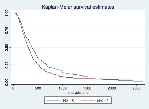
sts test sex
         failure _d:  status
   analysis time _t:  job_tenure


Log-rank test for equality of survivor functions

      |   Events         Events
sex   |  observed       expected
------+-------------------------
0     |       240         278.74
1     |       332         293.26
------+-------------------------
Total |       572         572.00

            chi2(1) =      10.64
            Pr>chi2 =     0.0011
Cox proportional hazard model
Next the PS asks for the estimation of a Cox proportional hazard model. You can estimate such model as follows:
stcox sex dex lex lex2
         failure _d:  status
   analysis time _t:  job_tenure

Iteration 0:   log likelihood = -3251.0092
Iteration 1:   log likelihood = -3143.0237
Iteration 2:   log likelihood = -3142.7797
Iteration 3:   log likelihood = -3142.7794
Refining estimates:
Iteration 0:   log likelihood = -3142.7794

Cox regression -- Breslow method for ties

No. of subjects =          683                     Number of obs   =       683
No. of failures =          572
Time at risk    =       276233
                                                   LR chi2(4)      =    216.46
Log likelihood  =   -3142.7794                     Prob > chi2     =    0.0000

------------------------------------------------------------------------------
          _t | Haz. Ratio   Std. Err.      z    P>|z|     [95% Conf. Interval]
-------------+----------------------------------------------------------------
         sex |   1.721651    .151811     6.16   0.000     1.448399    2.046454
         dex |   .9122404   .0060938   -13.75   0.000     .9003746    .9242625
         lex |   .3145531   .1027517    -3.54   0.000     .1658216    .5966875
        lex2 |   1.047419    .013782     3.52   0.000     1.020752    1.074783
------------------------------------------------------------------------------
In the output above, a hazard ratio equals one is the benchmark: if the hazard ratio is higher than one, the variable affects positively the hazard; if the hazard ratio is less than one, the variable contributes negatively to the hazard. This can be checked by asking for the coefficients rather than the proportional hazard rates representation of the Cox model:
stcox sex dex lex lex2, nohr
         failure _d:  status
   analysis time _t:  job_tenure

Iteration 0:   log likelihood = -3251.0092
Iteration 1:   log likelihood = -3143.0237
Iteration 2:   log likelihood = -3142.7797
Iteration 3:   log likelihood = -3142.7794
Refining estimates:
Iteration 0:   log likelihood = -3142.7794

Cox regression -- Breslow method for ties

No. of subjects =          683                     Number of obs   =       683
No. of failures =          572
Time at risk    =       276233
                                                   LR chi2(4)      =    216.46
Log likelihood  =   -3142.7794                     Prob > chi2     =    0.0000

------------------------------------------------------------------------------
          _t |      Coef.   Std. Err.      z    P>|z|     [95% Conf. Interval]
-------------+----------------------------------------------------------------
         sex |   .5432834   .0881776     6.16   0.000     .3704585    .7161084
         dex |  -.0918518     .00668   -13.75   0.000    -.1049444   -.0787592
         lex |  -1.156602   .3266594    -3.54   0.000    -1.796843   -.5163618
        lex2 |    .046329   .0131581     3.52   0.000     .0205397    .0721183
------------------------------------------------------------------------------
Please send comments to bottan2@illinois.edu or srmntbr2@illinois.edu↩