Data

You can download the data set, called weco14.csv from the Econ 508 web site. Save it in your preferred directory.

In the previous e-TA we cleaned, prepared and saved the data in Stata format. After setting the working directory to where the data is saved, lets open it:

   use weco14.dta, clear

Logit estimation

Here we estimate the same logit model proposed in question 3 of PS5

\[ logit(P(quit=1))= \beta_{0} + \beta_{1} sex + \beta_{2} dex +\beta_{3} lex + \beta_{4} lex^2 \]

where \(quit=1\) if the worker wuit withing the first 6 mothns after employment, and 0 otherwise.

To estimate this model first we need to create \(lex^2\).

   gen lex2 = lex^2

then we are ready to estimate the model. To do so we use the logit function


   logit kwit sex dex lex lex2

Iteration 0:   log likelihood = -372.98741  
Iteration 1:   log likelihood = -340.49246  
Iteration 2:   log likelihood = -339.21681  
Iteration 3:   log likelihood = -339.21165  
Iteration 4:   log likelihood = -339.21165  

Logistic regression                               Number of obs   =        683
                                                  LR chi2(4)      =      67.55
                                                  Prob > chi2     =     0.0000
Log likelihood = -339.21165                       Pseudo R2       =     0.0906

------------------------------------------------------------------------------
        kwit |      Coef.   Std. Err.      z    P>|z|     [95% Conf. Interval]
-------------+----------------------------------------------------------------
         sex |   .4655216   .1964162     2.37   0.018      .080553    .8504903
         dex |  -.1020059   .0147527    -6.91   0.000    -.1309207   -.0730911
         lex |  -1.967471   .6398749    -3.07   0.002    -3.221603   -.7133392
        lex2 |    .079972   .0255483     3.13   0.002     .0298982    .1300457
       _cons |   14.98417   4.080481     3.67   0.000     6.986576    22.98177
------------------------------------------------------------------------------

This is equivalent to estimate:

\[ Pr(kwit=1)=\frac{exp(x_{j} \beta)}{(1+exp(x_{j}\beta))} \]

The results above show that, ceteris paribus, workers with higher dexterity are less likely to quit, while males (sex=1) have a bigger tendency to quit than females (sex=0). In other words, positive coefficients contribute to increase the probability of quitting, while negative coefficients, to reduce it.

To draw a picture of the probability of quitting as a function of years of education, holding everything else constant (e.g., at their mean value), you need first to ask for mean of dexterity for the pooled sample, and then you can do it for males and females.

   sum dex
   local mean_dex = r(mean)
   sum dex if sex==1
   local mean_dex_male = r(mean)
   sum dex if sex==0
   local mean_dex_fem = r(mean)

Thus, let’s ask for the expected value of the probability of quitting conditioned to dexterity being hold at the pooled mean value:

   preserve
   replace dex = `mean_dex'
   predict p_hat
   scatter p_hat lex
   restore

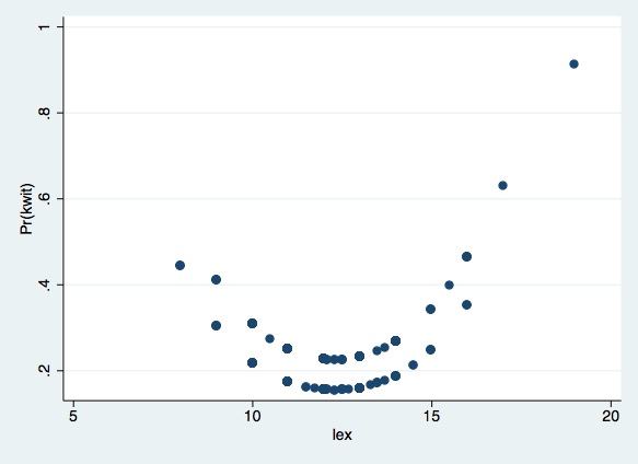
In the graph above you see two different curves -- one for male (upper curve) and another for female (lower curve). This happens because we left all explanatory variables constant at their means (in our case, only dex was fixed), but we had to leave sex  at its original values (because the average of the dummy variable does not make much sense in this case).

You can do this for males and females also. Next you are asked to examine better the effect of gender. A first suggestion is to tabulate sex and kwit:

   tab sex kwit

           |         kwit
       sex |         0          1 |     Total
-----------+----------------------+----------
         0 |       235         61 |       296 
         1 |       287        100 |       387 
-----------+----------------------+----------
     Total |       522        161 |       683 

In the table above you can see that 61 out of the existing 296 females in this sample are quitters, while 100 out of 387 males are quitters. So, the proportion of male quitters (56.6%) is greater than the proportion of female quitters (43.3%).

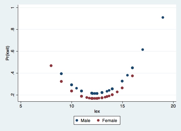
Next you can draw graphs of the expected probability of quitting for each gender, using their respective dexterity means. In R, we can ask for the graphs as follows:

   preserve
   replace dex = `mean_dex_male' if sex==1
   predict phat_male if sex==1
   replace dex = `mean_dex_fem' if sex==0
   predict phat_fem if sex==0
   twoway (scatter phat_male lex) (scatter phat_fem lex), legend(label(1 "Male") label(2 "Female"))
   restore

Besides the graphical analysis, you can also test for the shape of the education effect, by introducing the variables \(sex*lex\) and \(sex*lex2\) in the model, and checking their significance.

Next you are asked to evaluate the Logit specification by computing the Pregibon diagnostic. The first step is to generate the predicted probabilities of quitting, called p, and compute \(g_a\) (parameter that controls the fatness of tails) and \(g_d\) (parameter that controls symmetry):

   logit kwit sex dex lex lex2
   predict p
   gen ga=.5*(log(p)*log(p) - log(1-p)*log(1-p)) 
   gen gd=- .5*(log(p)*log(p) + log(1-p)*log(1-p)) 

Finally you run an extended Logit model, including the variables \(g_a\) and \(g_d\):

   logit kwit sex dex lex lex2 ga gd

Iteration 0:   log likelihood = -372.98741  
Iteration 1:   log likelihood =  -338.3799  
Iteration 2:   log likelihood = -337.12636  
Iteration 3:   log likelihood = -337.11333  
Iteration 4:   log likelihood = -337.11333  

Logistic regression                               Number of obs   =        683
                                                  LR chi2(6)      =      71.75
                                                  Prob > chi2     =     0.0000
Log likelihood = -337.11333                       Pseudo R2       =     0.0962

------------------------------------------------------------------------------
        kwit |      Coef.   Std. Err.      z    P>|z|     [95% Conf. Interval]
-------------+----------------------------------------------------------------
         sex |   .1048297   .5132355     0.20   0.838    -.9010934    1.110753
         dex |  -.0271078    .106906    -0.25   0.800    -.2366397    .1824241
         lex |   .1857418   2.322958     0.08   0.936    -4.367172    4.738656
        lex2 |   -.008141   .0945127    -0.09   0.931    -.1933824    .1771004
          ga |  -2.348945   1.946928    -1.21   0.228    -6.164854    1.466965
          gd |  -2.097206   1.422105    -1.47   0.140     -4.88448    .6900683
       _cons |  -1.084255   17.74923    -0.06   0.951     -35.8721    33.70359
------------------------------------------------------------------------------

And test their joint significance:

   test ga gd

 ( 1)  [kwit]ga = 0
 ( 2)  [kwit]gd = 0

           chi2(  2) =    3.26
         Prob > chi2 =    0.1958

The interpretation of the results is left to the reader.