
e-TA 13: Cubic B-Splines and Quantile Regression
Welcome to a new issue of e-Tutorial. This e-TA will focus on Cubic B-Splines and Quantile Regression.1
Data
You can download the data set, called weco14.csv from the Econ 508 web site. Save it in your preferred directory.
Then you can load it in Stata after setting your working directory to the folder where your downloaded the data by typing:
insheet using weco14.csv, cleardescribe
 Contains data
  obs:           683
 vars:             9
 size:        21,856
---------------------------------
              storage  display
variable name   type   format
---------------------------------
y               float  %9.0g
sex             byte   %8.0g
dex             byte   %8.0g
lex             float  %9.0g
kwit            str5   %9s
job_tenure      int    %8.0g
status          str5   %9s
treatment       str5   %9s
ypost           str5   %9s
--------------------------------
Note that some variables have been imported as strings. Let's see what is going on:
list in 1/5 +------------------------------------------------------------------------+
| y sex dex lex kwit job_te~e status treatm~t ypost |
|------------------------------------------------------------------------|
1. | 13.73 0 38 10 FALSE 277 TRUE TRUE 14.35 |
2. | 17.15 1 55 11 TRUE 173 TRUE NA NA |
3. | 13.63 1 45 12 FALSE 410 TRUE TRUE 15.75 |
4. | 13.04 1 41 11 FALSE 247 TRUE FALSE 18.33 |
5. | 13.2 1 42 10 FALSE 340 TRUE FALSE 13.96 |
+------------------------------------------------------------------------+
Notice that the variables that should be dummy variables (i.e. kwit,
status and treatment) are string, as well as ypost (missing values are
appearing as "NA". We will fix this using the destring function:
foreach var in kwit status treatment {
replace `var'="1" if `var'=="TRUE"
replace`var'="0" if `var'=="FALSE"
replace`var'="." if `var'=="NA"
destring `var', replace
}
destringypost, replace force
list in 1/5
* Save prepared data in Stata format
save weco14.dta, replace
     +-----------------------------------------------------------------------+
     |     y   sex   dex   lex   kwit   job_te~e   status   treatm~t   ypost |
     |-----------------------------------------------------------------------|
  1. | 13.73     0    38    10      0        277        1          1   14.35 |
  2. | 17.15     1    55    11      1        173        1          .       . |
  3. | 13.63     1    45    12      0        410        1          1   15.75 |
  4. | 13.04     1    41    11      0        247        1          0   18.33 |
  5. |  13.2     1    42    10      0        340        1          0   13.96 |
     +-----------------------------------------------------------------------+
Notice that all variables are now numeric and missing values are expressed with a ".".
Cubic B-Splines
First we begin by estimating the model proposed in question 1 of PS5
\[ y = \alpha_{0} + \alpha_{1} sex + \alpha_{2} dex + \alpha_{3} lex + \alpha_{4} lex^2 + u \]
To estimate this model first we need to create \(lex^2\)
gen lex2 = lex^2and then we are ready to estimate the model.
reg y sex dex lex lex2
      Source |       SS       df       MS              Number of obs =     683
-------------+------------------------------           F(  4,   678) =  107.52
       Model |  543.033017     4  135.758254           Prob > F      =  0.0000
    Residual |  856.087605   678  1.26266608           R-squared     =  0.3881
-------------+------------------------------           Adj R-squared =  0.3845
       Total |  1399.12062   682  2.05149651           Root MSE      =  1.1237

------------------------------------------------------------------------------
           y |      Coef.   Std. Err.      t    P>|t|     [95% Conf. Interval]
-------------+----------------------------------------------------------------
         sex |  -.9003615   .0874977   -10.29   0.000     -1.07216   -.7285625
         dex |   .1120702   .0060039    18.67   0.000     .1002818    .1238585
         lex |   .8219527   .3213372     2.56   0.011     .1910171    1.452888
        lex2 |  -.0360488   .0128092    -2.81   0.005    -.0611992   -.0108984
       _cons |   5.524386   2.032106     2.72   0.007     1.534408    9.514364
------------------------------------------------------------------------------
Next we estimate a “(more) nonparametric version” using Cubic B-Splines. To do so we will have to install it first:
ssc install bspline
Then we are ready to estimate a model of the form
\[ y = \alpha_{0} + \alpha_{1} sex + \alpha_{2} dex + g(lex, \alpha) + u \]
where \(g(.)\) is a spline. In Stata
we have to define the knots. To do so, we will arbitrarily choose 8,
12, 16, 19 (you should repeat trying different values) and we set the
power exponent equals to 3 (power of the spline). The bspline command will generate many variables with the name specified in gen( )
and a number at the end (for example, in our case it will generate
variables bs1, bs2, etc.). Finally, we run a Least Squares
regression including all the bspline variables generated and omit
lex (and lex squared) and omit the constant as well:
   sum lex, det

   bspline, xvar(lex) knots(8 12 16 19) gen(bs) power(3)
   reg y sex dex bs*, nocons
      Source |       SS       df       MS              Number of obs =     683
-------------+------------------------------           F(  8,   675) =14568.35
       Model |  147560.347     8  18445.0434           Prob > F      =  0.0000
    Residual |  854.620046   675  1.26610377           R-squared     =  0.9942
-------------+------------------------------           Adj R-squared =  0.9942
       Total |  148414.967   683  217.298634           Root MSE      =  1.1252

------------------------------------------------------------------------------
           y |      Coef.   Std. Err.      t    P>|t|     [95% Conf. Interval]
-------------+----------------------------------------------------------------
         sex |  -.8925394   .0879589   -10.15   0.000    -1.065245   -.7198335
         dex |   .1120716   .0060285    18.59   0.000     .1002348    .1239084
         bs1 |     13.327   4.844198     2.75   0.006     3.815496    22.83851
         bs2 |   9.372957   .7779693    12.05   0.000     7.845426    10.90049
         bs3 |   10.59208   .4503753    23.52   0.000     9.707771    11.47638
         bs4 |   9.549584   .6106413    15.64   0.000       8.3506    10.74857
         bs5 |   8.350974   2.087965     4.00   0.000     4.251287    12.45066
         bs6 |   4.851333   10.64133     0.46   0.649    -16.04276    25.74543
------------------------------------------------------------------------------
You can also plot the data with the regression spline overlain:
reg y bs*, noconspredict bspl
twoway (scatter y lex) (line bspl lex, sort)
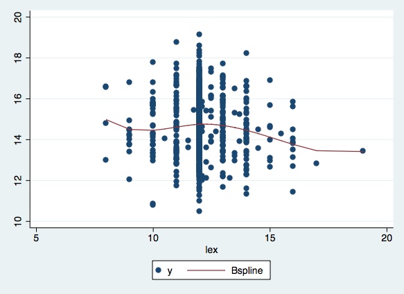
Note that we have defined new data where we are going to evaluate our estimates and used those to plot.
Quantile Regression
In Question 2 of PS5 we are asked to consider a quantile regression model that relates productivity, sex, dex and lex. For example we can think on a model of the form
\[ Q_{yi}(\tau|sex,dex,lex) = \alpha_0(\tau) + \alpha_1(\tau)sex_i +\alpha_2(\tau)+\alpha_3(\tau)lex_i+\alpha_4(\tau)lex_i ^2\]
where \(Q_{yi}(\tau|sex,dex,lex)\) is the \(\tau\)th conditional quantile. To estimate this model we use the qreg function, where as an option we define tau = 0.5 (i.e. the median):
qreg y sex dex lex lex2, q(.5)
Iteration  1:  WLS sum of weighted deviations =  610.25725

Iteration  1: sum of abs. weighted deviations =  610.87669
Iteration  2: sum of abs. weighted deviations =  610.14025
Iteration  3: sum of abs. weighted deviations =   609.9668
Iteration  4: sum of abs. weighted deviations =  609.92706
Iteration  5: sum of abs. weighted deviations =  609.80956
Iteration  6: sum of abs. weighted deviations =  609.80577
Iteration  7: sum of abs. weighted deviations =   609.8051
Iteration  8: sum of abs. weighted deviations =  609.80493

Median regression                                    Number of obs =       683
  Raw sum of deviations   790.26 (about 14.63)
  Min sum of deviations 609.8049                     Pseudo R2     =    0.2283

------------------------------------------------------------------------------
           y |      Coef.   Std. Err.      t    P>|t|     [95% Conf. Interval]
-------------+----------------------------------------------------------------
         sex |  -.8996744   .1175555    -7.65   0.000    -1.130491   -.6688578
         dex |   .1118793   .0080663    13.87   0.000     .0960413    .1277173
         lex |   .9100091   .4317253     2.11   0.035     .0623298    1.757688
        lex2 |  -.0398769   .0172094    -2.32   0.021    -.0736671   -.0060867
       _cons |   5.067943    2.73019     1.86   0.064    -.2927013    10.42859
------------------------------------------------------------------------------
If you want to estimate for several quantiles we can write:
sqreg y sex dex lex lex2, q(.1 .2 .3 .4 .5 .6 .7 .8 .9)(fitting base model)
(bootstrapping ....................)
Simultaneous quantile regression Number of obs = 683
bootstrap(20) SEs .10 Pseudo R2 = 0.1658
.20 Pseudo R2 = 0.1931
.30 Pseudo R2 = 0.2067
.40 Pseudo R2 = 0.2151
.50 Pseudo R2 = 0.2283
.60 Pseudo R2 = 0.2472
.70 Pseudo R2 = 0.2577
.80 Pseudo R2 = 0.2659
.90 Pseudo R2 = 0.2632
------------------------------------------------------------------------------
| Bootstrap
y | Coef. Std. Err. t P>|t| [95% Conf. Interval]
-------------+----------------------------------------------------------------
q10 |
sex | -.6510533 .2314608 -2.81 0.005 -1.105519 -.1965872
dex | .0968421 .011108 8.72 0.000 .0750319 .1186523
lex | .5460833 .7568564 0.72 0.471 -.9399809 2.032147
lex2 | -.0206692 .0278405 -0.74 0.458 -.0753331 .0339947
_cons | 5.657049 5.173943 1.09 0.275 -4.501828 15.81592
-------------+----------------------------------------------------------------
q20 |
sex | -.7770004 .1191531 -6.52 0.000 -1.010954 -.5430469
dex | .099 .0108908 9.09 0.000 .0776162 .1203837
lex | .5745001 .3655483 1.57 0.117 -.1432428 1.292243
lex2 | -.0240833 .0141285 -1.70 0.089 -.0518241 .0036574
_cons | 6.352584 2.438018 2.61 0.009 1.565611 11.13956
-------------+----------------------------------------------------------------
q30 |
sex | -.7418438 .1077119 -6.89 0.000 -.9533327 -.5303548
dex | .1060001 .0102943 10.30 0.000 .0857875 .1262128
lex | .7964917 .2455402 3.24 0.001 .3143812 1.278602
lex2 | -.0331587 .0092248 -3.59 0.000 -.0512713 -.0150461
_cons | 4.976792 1.671827 2.98 0.003 1.69421 8.259373
-------------+----------------------------------------------------------------
q40 |
sex | -.8249464 .1361408 -6.06 0.000 -1.092255 -.5576382
dex | .1093548 .0084511 12.94 0.000 .0927615 .1259482
lex | .8385486 .2595625 3.23 0.001 .3289058 1.348191
lex2 | -.0361828 .0095688 -3.78 0.000 -.0549709 -.0173947
_cons | 5.161289 1.860645 2.77 0.006 1.50797 8.814607
-------------+----------------------------------------------------------------
q50 |
sex | -.8996744 .1236826 -7.27 0.000 -1.142521 -.6568273
dex | .1118793 .0067787 16.50 0.000 .0985694 .1251891
lex | .9100091 .3438766 2.65 0.008 .2348181 1.5852
lex2 | -.0398769 .0135107 -2.95 0.003 -.0664048 -.013349
_cons | 5.067943 2.230586 2.27 0.023 .6882566 9.44763
-------------+----------------------------------------------------------------
q60 |
sex | -1.05875 .107784 -9.82 0.000 -1.27038 -.8471192
dex | .11375 .006795 16.74 0.000 .1004082 .1270917
lex | 1.012709 .3620856 2.80 0.005 .3017652 1.723653
lex2 | -.0444941 .0130878 -3.40 0.001 -.0701916 -.0187965
_cons | 4.835888 2.549023 1.90 0.058 -.1690398 9.840817
-------------+----------------------------------------------------------------
q70 |
sex | -1.014384 .0871026 -11.65 0.000 -1.185408 -.8433609
dex | .1203373 .0087235 13.79 0.000 .103209 .1374656
lex | .8846804 .4163887 2.12 0.034 .067114 1.702247
lex2 | -.0416624 .0147251 -2.83 0.005 -.0705746 -.0127501
_cons | 5.911409 2.979803 1.98 0.048 .0606577 11.76216
-------------+----------------------------------------------------------------
q80 |
sex | -.9837499 .0864969 -11.37 0.000 -1.153584 -.8139158
dex | .1187501 .0079648 14.91 0.000 .1031114 .1343888
lex | 1.105366 .3371336 3.28 0.001 .4434148 1.767317
lex2 | -.0507837 .0128111 -3.96 0.000 -.075938 -.0256294
_cons | 4.985955 2.321488 2.15 0.032 .4277845 9.544126
-------------+----------------------------------------------------------------
q90 |
sex | -1.193556 .157247 -7.59 0.000 -1.502305 -.8848059
dex | .1355703 .0115055 11.78 0.000 .1129795 .158161
lex | 1.228442 .571353 2.15 0.032 .1066077 2.350276
lex2 | -.0571591 .0226082 -2.53 0.012 -.1015495 -.0127686
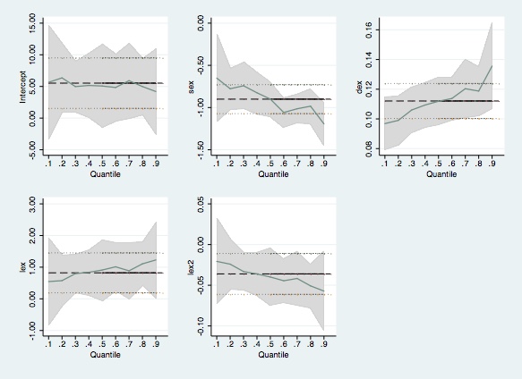
_cons | 4.200088 3.52878 1.19 0.234 -2.728562 11.12874
------------------------------------------------------------------------------grqreg, cons ci ols olsci
Please send comments to bottan2@illinois.edu or srmntbr2@illinois.edu↩