Econ 508
Econometrics Group
Home | Faculty | Students | Alumni | Courses | Research | Reproducibility | Lab | Seminars | Economics | Statistics | Fame
Applied Econometrics
Econ 508 - Fall 2007

e-Tutorial 9: Unit Roots and Cointegration

Welcome to the ninth issue of e-Tutorial. This issue focuses on time series models, with special emphasis on the tests of unit roots and cointegration. I am providing instructions for both R and STATA. I would like to remark that the theoretical background given in class is essential to proceed with the computational exercise below. Thus, I recommend you to study Prof. Koenker's Lectures 8 and 9 as you go through the tutorial.

First you need to download the data in text format by clicking here., or from the Econ 508 web site (Data).  Save it in your preferred directory (I will save my as "C:/eggs.txt".)  I suggest you to open the file in Notepad (or another text editor) and type the name of the variable "year" in the first row, first column, before "chic" "egg". Use <Tab> to separate the names of variables. Save the file (I will save mine as C:/eggs1.txt). 
 

Inserting the Data in R

Next, you need to import that data set to R, using the following commands:
Thurman<-read.table("C:/eggs1.txt", header=T)
year<-Thurman$year
egg<-Thurman$egg
chic<-Thurman$chic

It is useful to call the time series package, and declare chickens and eggs as time series:
library(ts)
year<-ts(year)
chic<-ts(chic)
egg<-ts(egg)
 

Inserting the Data in Stata:

In Stata, you can type:
infile year chic egg using"C:/eggs1.txt"

You will see that, because I included variables names in the first row of the file egg1.txt, Stata reads the first line of the data set as missing values. You should delete this line (only!) on the Stata data editor window. Next you need to declare your data as time series:
tsset year
 

I. Unit Root: Augmented Dickey-Fuller Test

At first, it is important that you to sketch the ADF test, explaining the NULL and the ALTERNATIVE hypotheses. 

ADF Test in R: I suggest you to use the R code adf.R, provided by Prof. Koenker, and available at http://www.econ.uiuc.edu/~econ472/routines.html:

#Copy from this point:
"adf"<-
function(x, L = 2, int = T, trend = T)
{
#Construct Data for Augmented Dickey Fuller Model with L lags.
#This is a modified version for R, in which the command rts was substituted by ts.
        x <- ts(x)
        D <- diff(x)
        if(L > 0) {
                for(i in 1:L)
                        D <- ts.intersect(D, lag(diff(x),  - i))
        }
        D <- ts.intersect(lag(x, -1), D)
        if(trend == T)
                D <- ts.intersect(D, time(x))
        y <- D[, 2]
        x <- D[, -2]
        if(int == T)
                summary(lm(y ~ x))
        else summary(lm(y ~ x - 1))
}
#To this point.
 

Your job is to copy the R code above and paste in the R console. This will create a R function called "adf", which runs the unit root test for each case. You should use the ADF test for each individual series (chickens and eggs), controlling for the number of lags, and the inclusion of constants and trends. 

Example 1:

#ADF for Chickens
#Model with 1 lag, constant and trend:
adf(chic, L=1, int=T, trend=T) 

Call:
lm(formula = y ~ x)

Residuals:
   Min     1Q Median     3Q    Max 
-52300 -11906  -2140   9191  77420 

Coefficients:
                        Estimate Std. Error t value Pr(>|t|) 
(Intercept)            8.360e+04  4.277e+04   1.955   0.0564 .
xD.lag(x, -1)         -1.821e-01  9.112e-02  -1.998   0.0514 .
xD.D.lag(diff(x), -i) -8.620e-02  1.435e-01  -0.601   0.5510 
xtime(x)              -3.156e+02  2.670e+02  -1.182   0.2429 
---
Signif. codes:  0 `***' 0.001 `**' 0.01 `*' 0.05 `.' 0.1 ` ' 1 

Residual standard error: 25030 on 48 degrees of freedom
Multiple R-Squared: 0.1067,     Adjusted R-squared: 0.05085 
F-statistic: 1.911 on 3 and 48 DF,  p-value: 0.1404 
 

Then you can test the significance of the coefficient xD.lag(x, -1)  by using the appropriate Dickey & Fuller critical values  (Table B.6 from Hamilton 1994, released in class). From this starting point, you can add lags by changing L=1 to L=2 or L=3 or L=4 and so on. If wish to exclude the intercept, just substitute int=T by int=F. (As usual, T means true, i.e., inclusion,  and F means false, i.e., exclusion). The same applies to the inclusion/exclusion of trend.

My suggestion is that you run 3 different types of ADF, each of them including 1, 2, 3, and 4 lags:
(i)   Models with intercept and trend (int=T, trend=T)
(ii)  Models with intercept but without trend (int=T, trend=F)
(iii) Models without intercept and without trend (int=F, trend=F)
 

Example 2:

#Model with 1 lag and constant, but not trend:
adf(chic, L=1, int=T, trend=F)

Call:
lm(formula = y ~ x)

Residuals:
   Min     1Q Median     3Q    Max 
-52968 -10923  -4082   9118  80473 

Coefficients:
                      Estimate Std. Error t value Pr(>|t|)
(Intercept)          5.198e+04  3.351e+04   1.551    0.127
xlag(x, -1)         -1.283e-01  7.926e-02  -1.618    0.112
xD.lag(diff(x), -i) -1.142e-01  1.421e-01  -0.803    0.426

Residual standard error: 25130 on 49 degrees of freedom
Multiple R-Squared: 0.08067,    Adjusted R-squared: 0.04314 
F-statistic:  2.15 on 2 and 49 DF,  p-value: 0.1274 
 

Example 3:

#Model with 1 lag, but no constant nor trend:
adf(chic, L=1, int=F, trend=F)

Call:
lm(formula = y ~ x - 1)

Residuals:
   Min     1Q Median     3Q    Max 
-60086 -11783  -1693  12188  77467 

Coefficients:
                     Estimate Std. Error t value Pr(>|t|)
xlag(x, -1)         -0.005967   0.008378  -0.712     0.48
xD.lag(diff(x), -i) -0.175791   0.138382  -1.270     0.21

Residual standard error: 25480 on 50 degrees of freedom
Multiple R-Squared: 0.03949,    Adjusted R-squared: 0.001073 
F-statistic: 1.028 on 2 and 50 DF,  p-value: 0.3652 
 

Do that for each individual series. This will generate 12 regressions for chickens, and 12 for eggs. Very likely, some of them will indicate the presence of unit root, while others will not. The choice of the best model can be done by calculating AIC, SIC or any other reasonable criterion. (See comments and analogy to OLS regressions in the respective STATA section.) At the end, please provide a table with the summary of your results, and draw your conclusions.
 

ADF Test in Stata: Once again, I recommend you to show explicitly what are the NULL and ALTERNATIVE hypotheses of this test, and the regression equations you are going to run. Then, using the STATA, you have two ways to perform the test: 

(1) using the command dfuller, or 
(2) using OLS (but checking for significance in the Dickey-Fuller tables). 

I suggest you to consider 3 variations of the test: 
(a) models with intercept and trend; 
(b) models with intercept, but without trend; 
(c) models without both intercept and trend.
 

A Simple Example: ADF in Stata:

a) Models including constant and trend: For example, using 1 lag in the chicken series, you will have the following result

dfuller  chic, regress trend lags(1)

Augmented Dickey-Fuller test for unit root         Number of obs   =        52

                               ---------- Interpolated Dickey-Fuller ---------
                  Test         1% Critical       5% Critical      10% Critical
               Statistic           Value             Value             Value
------------------------------------------------------------------------------
 Z(t)             -1.998            -4.146            -3.498            -3.179
------------------------------------------------------------------------------
* MacKinnon approximate p-value for Z(t) = 0.6030

------------------------------------------------------------------------------
D.chic   |      Coef.   Std. Err.       t     P>|t|       [95% Conf. Interval]
---------+--------------------------------------------------------------------
chic     |
      L1 |  -.1820551   .0911164     -1.998   0.051       -.365257    .0011467
      LD |  -.0861985   .1435294     -0.601   0.551      -.3747837    .2023867
_trend   |  -315.6405   266.9686     -1.182   0.243      -852.4168    221.1358
_cons    |   83287.07   42600.86      1.955   0.056      -2367.711    168941.8
------------------------------------------------------------------------------
 

Here the null hypothesis is the presence of unit root. Thus, the augmented Dickey-Fuller statistic is -1.998, and lies inside the acceptance region at 1%, 5%, and 10%. Therefore, we cannot reject the presence of unit root.
 

b) Models including constant but no trend: Same rationale, but adjusting the command to:

dfuller  chic, regress lags(1) 

Augmented Dickey-Fuller test for unit root         Number of obs   =        52

                               ---------- Interpolated Dickey-Fuller ---------
                  Test         1% Critical       5% Critical      10% Critical
               Statistic           Value             Value             Value
------------------------------------------------------------------------------
 Z(t)             -1.618            -3.577            -2.928            -2.599
------------------------------------------------------------------------------
* MacKinnon approximate p-value for Z(t) = 0.4737

------------------------------------------------------------------------------
D.chic   |      Coef.   Std. Err.       t     P>|t|       [95% Conf. Interval]
---------+--------------------------------------------------------------------
chic     |
      L1 |  -.1282545   .0792599     -1.618   0.112      -.2875333    .0310243
      LD |  -.1141494   .1421427     -0.803   0.426      -.3997958    .1714969
_cons    |   51982.91   33508.86      1.551   0.127      -15355.67    119321.5
------------------------------------------------------------------------------

What can you conclude from the null hypothes here?
 

c) Models excluding both constant and trend: Idem, but adjusting the command to:

dfuller  chic, noconstant regress lags(1)

Augmented Dickey-Fuller test for unit root         Number of obs   =        52

                               ---------- Interpolated Dickey-Fuller ---------
                  Test         1% Critical       5% Critical      10% Critical
               Statistic           Value             Value             Value
------------------------------------------------------------------------------
 Z(t)             -0.712            -2.619            -1.950            -1.610

------------------------------------------------------------------------------
D.chic   |      Coef.   Std. Err.       t     P>|t|       [95% Conf. Interval]
---------+--------------------------------------------------------------------
chic     |
      L1 |  -.0059671   .0083782     -0.712   0.480      -.0227951     .010861
      LD |  -.1757909   .1383822     -1.270   0.210      -.4537398     .102158
------------------------------------------------------------------------------

And here, what can you conclude?

Those equations regard unit root tests for the chickens annual series, using 1 lag. I recommend you to repeat these 3 processes for lags 2,3,and 4 as well. After you complete this cycle for chickens, you need to do the same cycle for eggs. At the end of both cycles, you will have 24 regression outputs. If you prefer, you don't need to report all output details, but rather concentrate on the ADF test statistics of each equation. You can do that by ommiting the term "regress" on the dfuller command. 
 

Presenting your ADF results:
Think that you are writing an academic paper. Don't spend too much space with intermediary results; concentrate instead on your final conclusions, which can be paradoxical as you go through different tetsting steps. By the end of the day you are expected to summarize your main results in a table, and then to write a paragraph with comments on the different results you can obtain when you include/exclude trends/constants/lags for both chickens and eggs series.
 

Comments on Unit Root Tests:

P.S.1: Unit root tests are very sensitive to the number of included lags and/or constant and trends. That's the reason by which we are asking you to show all ADF statistics in the table above. Very likely, some of the results will indicate the presence of unit root while others will not.

P.S.2: How to make a general conclusion on the test results with so many models available? Johnston & DiNardo (1997, p.226), for example, mention that one of the objectives of including lags is to achieve white noise residuals. Other authors recommend the use AIC or SIC in the model selection.

P.S.3: It is quite simple to calculate information criteria in ADF tests. Each output of "dfuller" corresponds to a linear regression on the lags, constant, and/or trend of the series (for a time trend, you can "approximate" the regression coefficient by using a vector from 1 to 54, instead of years). From OLS regression, you recover the sample size, the RSS, and the # of parameters requested to calculate SIC or AIC, plus the original ADF statistic. But remember to use the Dickey-Fuller critical values.

Example: The ADF test for unit root on the egg series, using 4 lags, but no constant nor trend is as follows:

dfuller  egg, noconstant regress lags(4)

Augmented Dickey-Fuller test for unit root         Number of obs   =        49
                               ---------- Interpolated Dickey-Fuller ---------
                  Test         1% Critical       5% Critical      10% Critical
               Statistic           Value             Value             Value
------------------------------------------------------------------------------
 Z(t)              1.033            -2.622            -1.950            -1.610
------------------------------------------------------------------------------
D.egg    |      Coef.   Std. Err.       t     P>|t|       [95% Conf. Interval]
---------+--------------------------------------------------------------------
egg      |
      L1 |    .005339    .005167      1.033   0.307      -.0050744    .0157524
      LD |   .3691248   .1547069      2.386   0.021       .0573335    .6809162
     L2D |  -.0210851   .1709519     -0.123   0.902       -.365616    .3234457
     L3D |  -.0248243   .1758323     -0.141   0.888      -.3791909    .3295423
     L4D |  -.0593437   .1599065     -0.371   0.712      -.3816141    .2629267
------------------------------------------------------------------------------

Similar output can be obtained by linear regression as follows:

 regress  D.egg L.egg LD.egg L2D.egg L3D.egg L4D.egg, noconstant

  Source |       SS       df       MS                  Number of obs =      49
---------+------------------------------               F(  5,    44) =    1.90
   Model |   275576.07     5  55115.2141               Prob > F      =  0.1144
Residual |  1278907.93    44  29066.0893               R-squared     =  0.1773
---------+------------------------------               Adj R-squared =  0.0838
   Total |  1554484.00    49  31724.1633               Root MSE      =  170.49
------------------------------------------------------------------------------
D.egg    |      Coef.   Std. Err.       t     P>|t|       [95% Conf. Interval]
---------+--------------------------------------------------------------------
egg      |
      L1 |    .005339    .005167      1.033   0.307      -.0050744    .0157524
      LD |   .3691248   .1547069      2.386   0.021       .0573335    .6809162
     L2D |  -.0210851   .1709519     -0.123   0.902       -.365616    .3234457
     L3D |  -.0248243   .1758323     -0.141   0.888      -.3791909    .3295423
     L4D |  -.0593437   .1599065     -0.371   0.712      -.3816141    .2629267
------------------------------------------------------------------------------
 

Did you understand why?

Note that the t-statistic for the lag of egg (L1) is the same as the ADF statistic, but the distribution used in the ADF hypothesis testing procedure is no longer the trivial t-student. Because of the unit root consequences, specific critical values are provided by Dickey and Fuller to test such statistic (Table B.6 from Hamilton 1994, released in class).
 

II. Cointegration: Engle-Granger Test

Here I recommend you to sketch the Engle-Granger test, explaining the NULL and the ALTERNATIVE hypotheses. :

Engle-Granger in R: The test can be done in 3 steps, as follows:

(i) Pre-test the variables for the presence of unit roots (done above) and check if they are integrated of the same order

(ii) Regress the long run equilibrium model of chickens vs. eggs

Engle<-lm(chic~egg)
summary(Engle)

Call:
lm(formula = chic ~ egg)

Residuals:
   Min     1Q Median     3Q    Max 
-49625 -30094 -13418  13555 166572 

Coefficients:
              Estimate Std. Error t value Pr(>|t|) 
(Intercept) 470461.481  36111.963  13.028   <2e-16 ***
egg            -10.219      7.133  -1.433    0.158 
---
Signif. codes:  0 `***' 0.001 `**' 0.01 `*' 0.05 `.' 0.1 ` ' 1 

Residual standard error: 45950 on 52 degrees of freedom
Multiple R-Squared: 0.03798,    Adjusted R-squared: 0.01948 
F-statistic: 2.053 on 1 and 52 DF,  p-value: 0.1579 

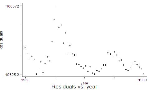
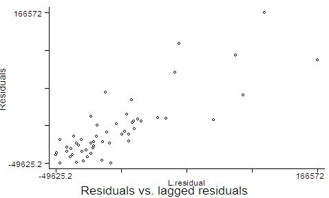
Obtain the residuals.

residual<-resid(Engle)

Plot the residuals along time.

ts.plot(year,residual, gpars=list(main="Chickens vs. eggs: Is there cointegration?", xlab="year", ylab="residuals"))

Plot also the residuals versus lagged residuals. Draw your conclusions

(iii) Test whether the residuals are I(0). (See discussion below in the respective STATA section).

At the end of the test, please provide a table summarizing your results. Comment your findings.
 

Engle-Granger in Stata: Follow the same 3 steps as above, with small software adjustments:

(i) Pre-test the variables for the presence of unit roots and check if they are integrated of the same order

(ii)Regress chickens against eggs (long run equilibrium relationship)

regress chic egg

  Source |       SS       df       MS                  Number of obs =      54
---------+------------------------------               F(  1,    52) =    2.05
   Model |  4.3347e+09     1  4.3347e+09               Prob > F      =  0.1579
Residual |  1.0981e+11    52  2.1117e+09               R-squared     =  0.0380
---------+------------------------------               Adj R-squared =  0.0195
   Total |  1.1414e+11    53  2.1536e+09               Root MSE      =   45953

------------------------------------------------------------------------------
    chic |      Coef.   Std. Err.       t     P>|t|       [95% Conf. Interval]
---------+--------------------------------------------------------------------
     egg |  -10.21917   7.132592     -1.433   0.158      -24.53176    4.093421
   _cons |   470461.5   36111.96     13.028   0.000       397997.5    542925.4
------------------------------------------------------------------------------

Obtain the residuals from this equation
predict residual, res

Graph the residuals against time
graph residual year, title(Residuals vs. year)


Graph the residuals against lagged residuals.
graph residual L.residual, title(Residuals vs. lagged residuals)


Draw your comments.

(iii) Proceed with a unit root test on the residuals, as you have done the ADF test for unit roots on chickens and eggs. Consider lags 0 to 4, though. This is a residual-based version of the ADF test. The only difference from the traditional ADF to (this version of) the Engle-Granger test are the critical values. The critical values to be used here are no longer the same provided by Dickey-Fuller, but instead provided by Engle and Yoo (1987) and others (see approximated critical values in Table B.9, Hamilton 1994). This happens because the residuals above are not the actual error terms, but estimated values from the long run equilibrium equation of chickens against eggs.

Some authors (e.g., Enders, 1995) consider a fourth step, consisting in the estimation of error-correction models and checking of models adequacy. However, you are not requiredto do that for the purposes of the problem set 3.


III. Cointegration: Johansen Test 

I recommend you to sketch the Johansen test, explaining the NULL and the ALTERNATIVE hypotheses. Then I suggest you to use the R code johansen.R, provided by Prof. Koenker, and available at http://www.econ.uiuc.edu/~econ472/routines.html:

#Copy from this point:
"johansen"<-
function(x, L = 2)
{
#Johansen Test of cointegration for multivariate time series x
#Returns vector of eigenvalues after that you are on your own.
#This is a modified version for R, in which rts is substituted by ts.
        x <- ts(x)
        n <- nrow(x)
        p <- ncol(x)
        Ly <- lag(x[, 1], -1)
        D <- diff(x[, 1])
        for(i in 1:p) {
                if(i > 1) {
                        D <- ts.intersect(D, diff(x[, i]))
                        Ly <- ts.intersect(Ly, lag(x[, i], -1))
                }
                if(L > 0)
                        for(j in 1:L)
                                D <- ts.intersect(D, lag(diff(x[, i]),  - j))
        }
        iys <- 1 + (L + 1) * (0:(p - 1))
        Y <- D[, iys]
        X <- D[,  - iys]
        Ly <- ts.intersect(Ly, D)[, 1:p]
        ZD <- lm(Y ~ X)$resid
        ZL <- lm(Ly ~ X)$resid
        df <- nrow(X) - ncol(X) - 1
        S00 <- crossprod(ZD)/df
        S11 <- crossprod(ZL)/df
        S01 <- crossprod(ZD, ZL)/df
        M <- solve(S11) %*% t(S01) %*% solve(S00) %*% S01
        eigen(M)$values
}
#To this point.

Your job is to copy the code above and paste in the R console. This will create a R function called "johansen" that calculates the eigenvalues. The command to obtain the eigenvalues is:

johansen(cbind(egg,chic), L=1)
[1] 0.16562116 0.05024913

The code above refers to the case including trend and intercept, and the appropriate critical values should be used. Note that the theoretical background here is essential, given that you need to interpret the eigenvalues and calculate the test statistic by yourself, before to draw your conclusions.


Johansen Test in Stata:
Stata 8 offers the possibility of testing for cointegration:


. tsset time

. vecrank egg chic


You should note that the eigenvalues are equal than before. Could you interpret the results? What is your conclusion?


 Last update: September 25, 2007