|
||||||
|
Applied Econometrics
e-Tutorial 6: Delta-Method and Bootstrap Techniques |
||||||
|
|
||||||
|
Welcome to the sixth issue of e-Tutorial, the on-line help to Econ 508. This issue provides an introduction on how to do the pratical works about the Delta-method and bootstrap in Stata and R. Hope this will be helpful for your further understanding of Prof. Koenker's Lecture 5 as well as the Question 4 of PS 2. I. Subtract Information from Tables in Stata and R. Running a Dynamic
Model with Quadratic and Multiplicative Terms gast = b0 + b1 incomet + b2 pricet + b3 (pricet)2 + b4 (pricet*incomet) + ut (A) Stata In Stata, you need first to generate the quadranic and other terms as follows: gen
price2= price^2 then run regressing: regress gas income price price2 priceinc Now, suppose you are asked to calculate the price elasticity of demand at different points of the sample. To do that you will need to: i) Obtain the coefficients of regression:
matrix B=get(_b) B[1,5]
ii) Extract the coefficients from the matrix B:
scalar b1=_coef[income]
Or another way to do it: scalar b1=B[1,1] iii) Calculate the elasticity at different points of the sample:
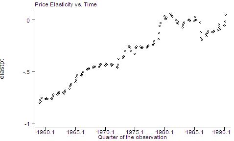
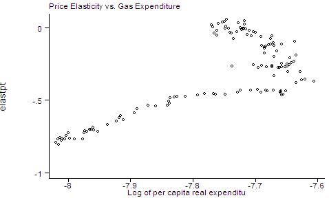
gen elastpt=b2+2*b3*price+b4*income iv) Ok. You've just created your elasticity series. Now you can study it at different points of the sample, plot it against year (check for inter-temporal structural breaks), against price, and against income. graph elastpt quarter, ylabel xlabel(1960.1 (5) 1990.1) t1title(Price Elasticity vs. Time)
graph elastpt gas, ylabel xlabel t1title(Price Elasticity vs. Gas Expenditure)
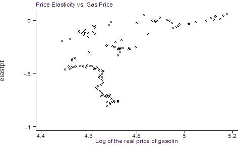
graph elastpt price, ylabel xlabel t1title(Price Elasticity vs. Gas Price)
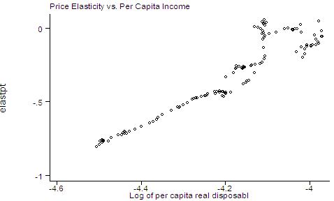
graph elastpt income, ylabel xlabel
t1title(Price Elasticity vs. Per Capita Income)
Remember that those are
point estimates. To compute confidence intervals, you will need special
techniques, as I'll show below (Delta-method and Bootstrap). Continuing with the problem set 2, question 4, you should: a) Interpret the implications of the model. b) Calculate the price
such that [b2+2*b3*price+b4*income] =
-1 c) Examine the partial residual plots (see Appendix A) d) Finally, in the last
part of the question 4 you are asked to estimate model 2 and to compute the
revenue maximizing price level assuming income=log(15)=2.708050
approximately. This is a straightforward computation. The interesting part
come with the application of the delta method and the bootstrap to achieve
reasonable confidence intervals for the optimal price. Standard Errors and Confidence Intervals for Non-linear Estimates: Delta-Method:You are expected to sketch the Delta-method and calculate the derivatives by hand along with the computational routine below. 1) Start running the full
model again:
Source |
SS df
MS
Number of obs = 128 ------------------------------------------------------------------------------
2) Recall that you have stored those coefficients under the names [b1, b2 , b3, b4, b0]. Now you need to get the covariance matrix V of them: matrix
V=get(VCE) Please note the order of the covariance matrix: the first column corresponds to the coefficient of income, the second to the coefficient of price, the third to the coefficient of price2, the fourth to the coefficient of priceinc, and the last to the coefficient of the intercept _cons. See the results below: symmetric
V[5,5] 3) Next you need to input
pstar: 4) And then you need to obtain the gradient vector with the partial derivatives of pstar (optimal price) with respect to each regressor, obeying the order of the covariance matrix: G'= (dpstar/d_coef[income],
which is the same as G'= (dpstar/db1 , dpstar/db2, dpstar/db3, dpstar/db4, dpstar/db0) In STATA the vector will be as follows: matrix
G=( 0 \ -1/(2*b3) \ (1+b2+b4*ln(15))/(2*b3*b3)
\ -ln(15)/(2*b3) \ 0) This corresponds to the gradient vector. The backslashes separate each row of the vector. The results are as follows: G[5,1]
5) The next step is to obtain the estimated variance of the optimal price, G'VG: matrix GVG=G'*V*G symmetric
GVG[1,1] 6) Then you can obtain
the standard error by taking the square root of this scalar value: sepstar = 13.236079 That's it. The variable sepstar
is the standard error of pstar. 7) The last step is to construct your confidence interval, and put the variables in levels, as follows: scalar
CIupper=pstar + 1.96*sepstar This will give you the
confidence interval of the optimal price level. Observe that the results you
obtained are for prices in logs. You can try to get the respective results in
levels as well, but it is worth to think about whether you can do that
directly or you need some additional step because of the non-linearity of the
point estimate. Bootstrap: You are expected to explain the various Bootstrap techniques in words (as if you are explaining for a non-econometrician), along with the complete understanding of the results provided by STATA. In STATA, you can calculate parametric (Normal), percentiled, and bias corrected bootstrapped confidence intervals for the optimal price as follows: set
seed 1 command:
reg gas income price price2 priceinc Bootstrap statistics Variable
| Reps Observed
Bias Std. Err. [95% Conf. Interval] In the command above, you use set seed 1 to assure reproducibility of your results. It means that, instead of generating a different initial random number every time you run the bootstrap, STATA will use the same seed, i.e., same initial random number (equals 1 in this case), for the iteration process. The first expression in quotation marks is the estimator, while the second quoted expression is the estimate you are interested. reps (10000) means that STATA will repeat the process 10000 times, to give you the confidence interval. Recall the generated
statistic is in log form. A good question is whether you should present your
Delta-method and Bootstrap confidence interval in logs or in levels... Think
about it. Appendix A: Partial Residual Plot Revisited It is importante to mention that all results presented here are based on a different data set (auto2.dta) than the data set used on the problem set 2 (gasnew.dat): I) Use the partial residual plot to check on the effect of the quadratic term. To obtain the partial residual plot with respect to the quadratic term you should :
I.1) Estimate model (2) without the regressor price2, and call this model
(2.1)
Source |
SS df
MS
Number of obs = 128 ------------------------------------------------------------------------------
I.2) Obtain the residuals of the
model (2.1):
I.3) Estimate
model (2) using price2 instead of gas as the dependent variable; call it
model (2.2):
Source |
SS df
MS
Number of obs = 128 ------------------------------------------------------------------------------
I.4) Obtain the
residuals of the model (2.2):
I.5) Run the
Gauss-Frisch-Waugh "regression", and check if the slope coefficient
is the same as in the original model (2):
Source |
SS df
MS
Number of obs = 128 ------------------------------------------------------------------------------
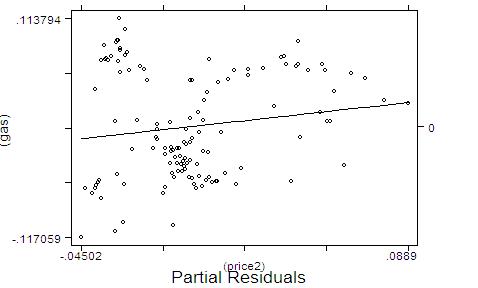
I.6) Plot the the partial residuals, with a fitting line of predicted values
(here called gfw):
II) Check whether there is a linear relationship between the residuals of the model (2.1) and the residuals of model (2.2). Draw your conclusion from what you see in the graph, and try to justify your answer in the light of basic assumptions of linear regression. USING R: Delta-Method: 1) Infile the data,
transform them in time series, and run the full model d.gas<-read.table("http://www.econ.uiuc.edu/~econ472/AUTO2.txt",header=T) attach(d.gas) gas<-ts(gas,start=1959,frequency=4) price<-ts(price,start=1959,frequency=4) income<-ts(income,start=1959,frequency=4) miles<-ts(miles,start=1959,frequency=4) price2<-price^2 princ<-price*income f<-lm(gas~income+price+price2+princ) summary(f) coefs<-f$coefficients 2) Recall
that you have stored those coefficients under the names [b0, b1,
b2 , b3, b4] anf constant term comes first.
Now you need to get the covariance matrix V of them vc<-vcov(f) 3) Next you need to input
pstar: pstar
<- (-(1+coefs[3]+coefs[5]*log(15))/(2*coefs[4]) ) pstar 4) And then you need to obtain the gradient vector with the partial derivatives of pstar (optimal price) with respect to each regressor, obeying the order of the covariance matrix: G'= (dpstar/d_coef[ _cons] dpstar/d_coef[income],
which is the same as G'= (dpstar/db0,dpstar/db1 , dpstar/db2, dpstar/db3, dpstar/db4) In R one could do this as follows: First generate a vector containig the values g<-c(0,0,-1/(2*coefs[4]),(1+coefs[3]+coefs[5]*log(15))/(2*coefs[4]*coefs[4]), -log(15)/(2*coefs[4])) g Then generate the matrix G<-matrix(g,ncol=1,nrow=5) G > G [,1] [1,] 0.000000 [2,] 0.000000 [3,] -1.761006 [4,] 49.792894 [5,] -4.768893 5) The next step is to obtain the estimated variance of the optimal price, G'VG: Var<-t(G)%*%vc%*%G Var [,1] [1,] 175.1848 6) Then you can obtain
the standard error by taking the square root of this scalar value: se.pstar<-sqrt(Var) se.pstar > se.pstar [,1] [1,] 13.23574 That's it. The variable se.pstar
is the standard error of pstar. 7) The last step is to construct your confidence interval, and put the variables in levels, as follows: Ciupper<-pstar + 1.96*se.pstar pstar Cilower > Ciupper [,1] [1,] 11.80442 > pstar
price -14.13763 > Cilower [,1] [1,] -40.07967 Bootstrap: For Bootstrap we use the two codes provide in the Lecture
notes 5. rm(list=ls() d.gas<-read.table("http://www.econ.uiuc.edu/~econ472/AUTO2.txt",header=T) attach(d.gas) gas<-ts(gas,start=1959,frequency=4) price<-ts(price,start=1959,frequency=4) income<-ts(income,start=1959,frequency=4) miles<-ts(miles,start=1959,frequency=4) price2<-price^2 princ<-price*income CODE
1 FOR BOOTSTRAP: fit.star<-lm(gas~income+price+price2+princ) uhat<-fit.star$resid R<-1000
# Number of Repetions h<-rep(0,R) for
(i in 1:R){ gash<-fit.star$fit+sample(uhat,replace=TRUE) b<-lm(gash~income+price+price2+princ)$coef h[i]<-
(-(1+b[3]+b[5]*log(15))/(2*b[4])) }
quantile(h,c(0.025,0.975)) >
quantile(h,c(0.025,0.975)) 2.5% 97.5% -123.5313 72.2807 CODE
2 FOR BOOTSTRAP: n<-length(gas) R<-1000
# Number of Repetions a<-rep(0,R) for
(i in 1:R){ s<-sample(1:n,replace=TRUE) f<-lm(gas[s]~income[s]+price[s]+price2[s]+princ[s]) coefs<-f$coefficients a[i]<-(-(1+coefs[3]+coefs[5]*log(15))/(2*coefs[4])) }
quantile(a,c(0.025,0.975)) >
quantile(a,c(0.025,0.975)) 2.5% 97.5% -125.77590 94.38562
|
||||||
|
|
||||||
|
|
|
Last update: September 12, 2007 |