|
||||||||||||||||||||||||||||||||||||||||||||||||
|
Applied Econometrics
e-Tutorial 4: Introduction to Dynamic Models |
||||||||||||||||||||||||||||||||||||||||||||||||
|
|
||||||||||||||||||||||||||||||||||||||||||||||||
|
Welcome to the fourth issue of e-Tutorial, the on-line help to Econ 508. This issue provides an introduction to dynamic models in Econometrics, and draws on Prof. Koenker's Lecture Note 3. The adopted philosophy is "learn by doing": the material is intended to help you to solve the problem set 2 and to enhance your understanding of the topics. Data Set: quarter
Quarter of the observation (from 1959.1 to 1990.4) Summarizing the data
summarize Variable
| Obs
Mean Std. Dev.
Min Max Even better, you can ask for the details of each variable: summarize, detail
Quarter of the observation 50%
1974.75
Mean
1974.75
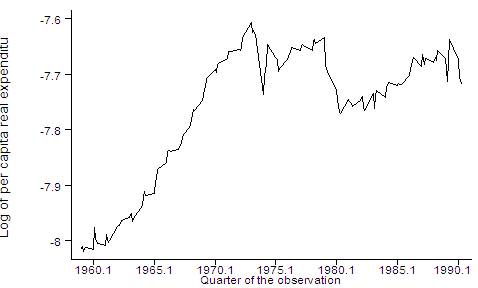
Log of per capita real expenditure on gasoline and 50%
-7.719422
Mean -7.763027
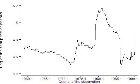
Log of the real price of gasoline and oil 50%
4.675815
Mean 4.723974
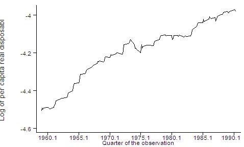
Log of per capita real disposable income 50%
-4.158388
Mean -4.19457
Log of miles per gallon 50%
2.64715
Mean 2.712568
Generating Lags,
Leads, and Differences: Usually the strategy (ii) saves you time during the model selection process. Hence, following (ii), you need to generate a variable corresponding to the time period of each observation (which can not be “quarter” because it contains non-integer values): gen
t=_n Next you
"tsset" your data using the created variable: Now you are ready to work
with time series. The main operators you will need are:
The remaining
lags/leads/differences can be generated using combination of the operators
above. Graphing Time Series:
graph gas quarter, c(l) s(.) sort ylabel xlabel(1960.1 (5) 1990.1)
graph price quarter, c(l) s(.) sort ylabel xlabel(1960.1 (5) 1990.1)
graph income quarter, c(l) s(.) sort ylabel xlabel(1960.1 (5) 1990.1)
Running Dynamic Models: Next let’s run a typical dynamic model (Johnston and DiNardo, 1997, p. 269, Table 8.5): regress
gas price L.price L2.price L3.price L4.price L5.price income
L.income L2.income L3.income L4.income L5.income L.gas L2.gas L3.gas
L4.gas L5.gas
Source |
SS df
MS
Number of obs = 123 ------------------------------------------------------------------------------
Long-run Elasticities: Suppose you wish to compute the long run income and price elasticities. Assuming that in the long-run the variables converge to their respective steady-state values (represented by “e”): gas(t)=gas(t-1)=gas(t-2)=...=gas(e)
and recalling that all variables are already in logs, you then just have to apply this steady state condition, reparameterize the model, and calculate the elasticities: d
(gas(e))/ d (income(e))= long run income elasticity After that you can compare the long-run elasticities of the (reparameterized) dynamic model with the elasticities provided by the static version of this log-linear regression: regress gas price income
Source |
SS df
MS
Number of obs = 128 ------------------------------------------------------------------------------
I suggest you to provide a little table comparing those results, and write your comments about how the elasticities differ from the static to the dynamic model. In the light of the
problem set 1, I suggest you to compute not only the point estimate of the
elasticities, but also their confidence intervals. In the static model,
confidence intervals are obtained directly from the regression output. But
for the dynamic model, the elasticities are represented by a non-linear
function of the parameters. In that case, you need to find confidence
intervals for the elasticities using Delta-method or Bootstrap techniques,
which you will see in professor Koenker’s lecture Note 4. Impulse Response Functions: Here I recommend to use the best dynamic model (following the Schwarz Information Criterion that you will see in e-Tutorial 5), and to compute impulse response functions using the formula on Prof. Koenker's Lecture Note 3, page 3. P.S.: Some authors propose alternative ways to calculate impulse response functions. One of them is to use partial derivatives (e.g., Enders, 1995, p.24), but such method has a drawback: it is quite easy to make a mistake when you have models with many lags and differences. Usually it is expected
that you account for a reasonable amount of response periods, depending on
the structure of your data set. Usually we suggest a minimum of 40 (forty)
response periods for quarterly data. Then you plot those responses along the
respective time scale (t=0,1,2,3,...,40). This will generate the
non-cumulative impulse response function. If you wish a cumulative impulse
response function, at each new period t+i (i=1,2,3,...), you should add the
effect to the previous shocks. Error Correction Model (ECM): There is no mystery in
doing that. You just have to add and subtract y(t-1) and \beta_{0}*x(t-1)
on the model, reparameterize it, and obtain a dynamic equation in which the
difference of the response (dependent) variable is decomposed into two parts:
(a) direct effects from changes in the explanatory variables, and (b)
indirect effects from changes on the response variable during previous
periods, while it was out-of-equilibrium. (See, for example, Prof. Koenker’s
Lecture Note 3, p. 5.) Using R: In order to estimate a time
series model in R we need to transform the data in “time series” first. We
can do that we loagind two libraries, say stats and dyn. library(stats) library(dyn) Let’s see the example for the gasoline data. Infile the data: d.gas<-read.table("http://www.econ.uiuc.edu/~econ472/data/AUTO2.txt",header=T) attach(d.gas) gas<-ts(gas,start=1959,frequency=4) price<-ts(price,start=1959,frequency=4) income<-ts(income,start=1959,frequency=4) miles<-ts(miles,start=1959,frequency=4) Now, we are ready to run regressions. One could run, for example: f<-dyn$lm(gas~lag(gas,-1)+price) summary(f) Call: lm(formula = dyn(gas ~ lag(gas, -1)
+ price)) Residuals: Min
1Q
Median 3Q
Max -0.1070295 -0.0071226 0.0003278 0.0105659
0.0359612 Coefficients:
Estimate Std. Error t value Pr(>|t|) (Intercept) -0.129960 0.115034
-1.130 0.2608 lag(gas, -1) 0.970998 0.013543
71.697 <2e-16
*** price -0.019652 0.009811 -2.003 0.0473 *
--- Signif. codes: 0 '***' 0.001 '**' 0.01 '*' 0.05 '.'
0.1 ' ' 1 Residual standard error: 0.01833 on
124 degrees of freedom Multiple R-Squared: 0.9765, Adjusted R-squared:
0.9761 F-statistic: 2572 on 2 and 124 DF, p-value: < 2.2e-16 In order to do differences, just type f2<-dyn$lm(gas~lag(gas,-1)+price+lag(diff(gas),-1)) summary(f2) Call: lm(formula = dyn(gas ~ lag(gas, -1)
+ price + lag(diff(gas), -1))) Residuals: Min
1Q
Median 3Q
Max -0.1081008 -0.0075195 0.0006098 0.0113212
0.0398956 Coefficients:
Estimate Std. Error t value Pr(>|t|) (Intercept)
-0.12594
0.11686 -1.078 0.2833 lag(gas, -1)
0.96955
0.01379 70.289 <2e-16 *** price -0.02281 0.01007 -2.265 0.0253 *
lag(diff(gas), -1) -0.12166 0.08928 -1.363 0.1755 --- Signif. codes: 0 '***' 0.001 '**' 0.01 '*' 0.05 '.'
0.1 ' ' 1 Residual standard error: 0.01833 on
122 degrees of freedom Multiple R-Squared: 0.976, Adjusted
R-squared: 0.9754 F-statistic: 1652 on 3 and 122 DF, p-value: < 2.2e-16 If you want to reproduce
the dynamic model given by Johnston and DiNardo, 1997, p. 269, Table 8.5,
just type f3<-dyn$lm(gas~price+lag(price,-1)+
lag(price,-2)+ lag(price,-3)+ lag(price,-4)+ lag(price,-5)+income+lag(income,-1)+
lag(income,-2)+ lag(income,-3)+ lag(income,-4)+lag(income,-5)+lag(gas,-1)+
lag(gas,-2)+ lag(gas,-3)+ lag(gas,-4)+ lag(gas,-5)) summary(f3) and you get the same model as described above.
|
||||||||||||||||||||||||||||||||||||||||||||||||
|
|
|
Last update: Sep. 9, 2008 |