e-Tutorial 2: A Brief Introduction to R

What's R?
"R is a system for statistical computation and graphics. It consists of a language plus a run-time environment with graphics, a debugger, access to certain systems functions, and the ability to run programs stored in script files." (The R FAQ, by Kurt Hornink (2001), http://www.ci.tuwien.ac.at/~hornik/R/ ).

Accessing R
R is currently available at the Econometrics Lab, DKH, for students enrolled in the Econometrics field or other classes that require lab experiments. You can also obtain a free copy of R at the main mirrors of the CRAN (Comprehensive R Archive Network) on the web, indicated in the FAQ material above, or download it using the archive of R introductory materials available at the UIUC Statistics Department web site (see below).

Installing R (Windows Version)
To install the software, just follow these steps:
i)    Go to http://cran.r-project.org/
ii)   Click link Windows (95 or later), then click link base.
iii)  Download the installer rw1091.exe.
iv)  Disable Viruscan before installing. Then click on the installer wizard.
v)   Change destination to an appropriate sub directory of "Program Files", e.g., ../Program Files/R.
vi)  Save all manuals in a .pdf format such that you can read it on-line.
vii) Search for the file RGui.exe in your computer, and create a shortcut to it. To begin working in R, just run RGui.exe.

Useful Links
CRAN : R Archive
R Homepage
Introduction to R : Introductory document for R
R for Octave users : R-Octave translation page
R for Matlab users : R-Matlab translation document

Downloading Data
There are many ways to download data in R. (For detailed info, please type help(read.table) and press <enter> in the R Console). Here I suggest the use of .csv (comma delimited) format. The best way to learn about that is through a simple example as follows.

Example - The U.S. Economy in the 1990s
Let's start with an analysis of the performance of the U.S. economy during the 1990s. I have collected annual data on GDP growth, GDP per capita growth, private consumption growth, investment growth, manufacturing labor productivity growth, unemployment rate, and inflation rate. (The data is publicly available in the statistical appendixes of the World Economic Outlook, May 2001, IMF). The first two variables can be seen as dependent variables, and you should test whether they are close substitutes. Consumption, investment, and productivity can be seen as factors that enhance GDP growth, and therefore you should expect positive covariates for those variables. Finally, unemployment and inflation rates are intrinsically correlated, and you should check whether any (or both) can be included in our simplistic growth model.

To download the data, please follow the general steps below:
a) Go to the web page containing the data (click here to access the data in a text format), and save it.
b) After saving, go to Microsoft Excel and open the file. (If a "Text Import Wizard" window pops up, just press "Next".)
c) Insert a row before the first line containing data.
d) Type the title of each column (variable) on that new row you have inserted.
e) Save the file as .csv in your Econ508 directory, e.g., "C:/Econ508/US90.csv". Close MS Excel.
f) Open Notepad (or any text editor) and type the following commands:

  US90<-read.csv("C:/Econ472/US90.csv", header=T)
  year<-US90$year
  gdpgr<-US90$gdpgr
  consgr<-US90$consgr
  invgr<-US90$invgr
  unemp<-US90$unemp
  gdpcapgr<-US90$gdpcapgr
  inf<-US90$inf
  producgr<-US90$producgr

Save the file as US90code.txt.  This will create a routine to download the data. Here you are naming the data set as "US90" and asking R to import it from the file "US90.csv" located in the directory "C:/Econ508/". The term "header" refers to the names of the variables in the first row. The lines 2-9 corresponds to each individual variable - in order to work with them, you need to extract them from the data frame (single object) and give respective names after that (multiple objects).
 

f) Start R (i.e., run RGui.exe). In the toolbar, go to "File", "Source R code", and open the file US90code.txt containing your routine.  (Be careful to name the right directory where you have saved your routine.)
 

g) In the window called R Console, type US90. You will be able to see the matrix containing the data (a.k.a. data frame). If you type the name of a single variable, you will be able to visualize that on the screen as a vector.

Now you are ready to work with your data!!

Basic Operations
A useful way to explore your data is checking the main statistics of each variable. For example, in the R Console window you can obtain the minimum, 1st quartile, median, 3rd quartile, and maximum of each variable in your data set by typing
summary(US90)

If you also wish to know the standard deviation of the series, type
sd(US90)

If you are only interested in a single variable, just include its name after the command
summary(gdpgr)
sd(gdpgr)

If you are in interested only in subset of your data, you can inspect it using filters. For example, begin by checking the dimension of the data matrix:
dim(US90)
 [1] 11  8

This means that your data matrix contains 11 rows (corresponding to the years 1992 to 2002) and 8 columns (corresponding to the variables). If you are only interested in a subset of the time periods (e.g., the years of the Clinton administration), you can select it as a new object:
Clinton<-US90[2:9, ]

and then compute its main statistics:
summary(Clinton)

If you are only interested in a subset of the variables (e.g., consumption and investment growth rates), you can select them by typing:
VarSet1<-US90[ ,3:4]

and then compute its main statistics:
summary(VarSet1)

To create new variables, you can use traditional operators (+,-,*,/,^) and name new variables as follows:

add or subtract:  lagyear<-year-1
multiply:       newgdpgr<-gdpgr*100
divide:         newunemp<-unemp/100
exponential:    gdpcap2<-gdpcapgr^2
square root:      sqrtcons<-sqrt(consgr)
natural logs:     loginv<-log(invgr)
base 10 logs:     log10inf<-log10(inf)
exponential:    expprod<-exp(producgr)

Last, but not least, the Help command (e.g., type help("log") in the R Console) contains short but useful information on the main packages with functions provided by R. Later in Econ508, you will learn how to create your own functions in R.
 

Exploring Graphical Resources

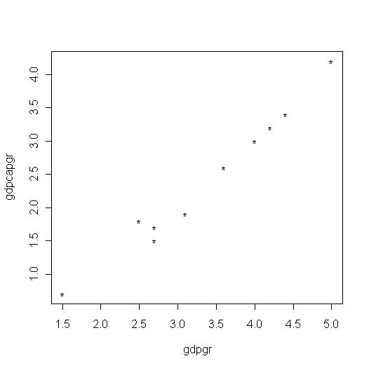
Suppose now you want to check the relationship among variables. For example, suppose you would like to see how much GDP growth is related with GDP per capita growth. This corresponds to a single graph that could be obtained as follows:
plot(gdpgr, gdpcapgr, pch="*")

And the result will be:
 
 

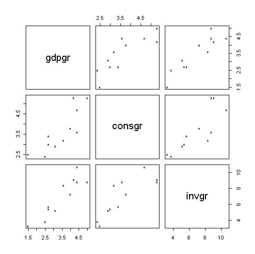
Another useful tool is the check on multiple graphs in a single window. For example, suppose you would like to expand your selection, and  check the pair wise relationship of GDP, Consumption, and Investment Growth. You can obtain that as follows:
pairs(US90 [, 2:4], pch="*")

The result will be:

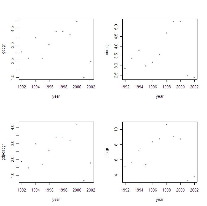
Suppose you would like to see the performance of multiple variables (e.g., GDP, GDP per capita, Consumption, and Investment growth rates) along time. The simplest way is as follows:

par(mfrow=c(2,2))
plot(year, gdpgr,    pch="*")
plot(year, consgr,   pch="*")
plot(year, gdpcapgr, pch="*")
plot(year, invgr,    pch="*")

Here the command "par(mfrow=c(2,2))" creates a matrix with 2 rows and 2 columns in which the individual graphs will be stored, while the command "plot" is in charge of producing individual graphs for each selected variable. The output will be:

You can easily expand the list of variables to obtain a graphical assessment of the performance of each of them along time. You can also use the graphs to assess cross-correlations (in a pair wise sense) among variables.
 
 

Linear Regression

Before running a regression, it is recommended you check the cross-correlations among covariates. You can do that graphically (see above) or using the following simple command:
cor1<-cor(US90)
cor1

The output will be:

> c1
                year       gdpgr     consgr       invgr      unemp   gdpcapgr
year      1.00000000 -0.02868877  0.1311224 -0.03003992 -0.8708412  0.1064203
gdpgr    -0.02868877  1.00000000  0.8393692  0.90974640 -0.3034902  0.9890287
consgr    0.13112235  0.83936925  1.0000000  0.82695132 -0.4761100  0.8347306
invgr    -0.03003992  0.90974640  0.8269513  1.00000000 -0.3684201  0.8841040
unemp    -0.87084123 -0.30349017 -0.4761100 -0.36842005  1.0000000 -0.4143217
gdpcapgr  0.10642030  0.98902873  0.8347306  0.88410398 -0.4143217  1.0000000
inf      -0.33598498 -0.10120944 -0.1198435 -0.30902448  0.3590237 -0.1229620
producgr  0.33166789  0.57079980  0.7049924  0.52383121 -0.5336310  0.6002807
                 inf    producgr
year     -0.33598498  0.33166789
gdpgr    -0.10120944  0.57079980
consgr   -0.11984349  0.70499242
invgr    -0.30902448  0.52383121
unemp     0.35902370 -0.53363102
gdpcapgr -0.12296202  0.60028067
inf       1.00000000 -0.08321976
producgr -0.08321976  1.00000000
>

From the matrix above you can see, for example, that GDP and GDP per capita growth rates are closely related, but each of them has a different degree of connection with unemployment rates (in fact, GDP per capita presents higher correlation with unemployment rates than total GDP). Inflation and unemployment present a reasonable degree of positive correlation (about 36%).

Now you start with simple linear regressions. For example, let's check the regression of GDP versus investment growth rates. You just type:
model1<-lm(gdpgr~invgr)
summary(model1)

And the output will be:

Call:
lm(formula = gdpgr ~ invgr)

Residuals:
    Min      1Q  Median      3Q     Max
-0.5503 -0.3515 -0.1152  0.3106  0.8039

Coefficients:
            Estimate Std. Error t value Pr(>|t|)
(Intercept)  0.70328    0.44220   1.590 0.146208
invgr        0.39691    0.06038   6.574 0.000102 ***
---
Signif. codes:  0  `***'  0.001  `**'  0.01  `*'  0.05  `.'  0.1  ` '  1

Residual standard error: 0.4599 on 9 degrees of freedom
Multiple R-Squared: 0.8276,     Adjusted R-squared: 0.8085
F-statistic: 43.22 on 1 and 9 degrees of freedom,       p-value: 0.0001023
 

Please note that you don't need to include the intercept, because R automatically includes it. In the output above you have the main regression diagnostics (F-test, adjusted R-squared, t-statistics, sample size, etc.). The same rule apply to multiple linear regressions. For example, suppose you want to find the main sources of GDP growth. The command is:

model2<-lm(gdpgr~consgr+invgr+producgr+unemp+inf)
summary(model2)

And the output is:

Call:
lm(formula = gdpgr ~ consgr + invgr + producgr + unemp + inf)

Residuals:
       1        2        3        4        5        6       7        8
 0.09515 -0.37843  0.40786 -0.16802 -0.33377  0.43903 -0.26519 -0.19791
       9       10       11
 0.28562 -0.43586  0.55152

Coefficients:
            Estimate Std. Error t value Pr(>|t|)
(Intercept) -0.88659    1.49293  -0.594   0.5785
consgr       0.18221    0.36052   0.505   0.6348
invgr        0.34489    0.13380   2.578   0.0496 *
producgr     0.04902    0.15473   0.317   0.7642
unemp        0.05517    0.18980   0.291   0.7830
inf          0.30196    0.37260   0.810   0.4545
---
Signif. codes:  0  `***'  0.001  `**'  0.01  `*'  0.05  `.'  0.1  ` '  1

Residual standard error: 0.517 on 5 degrees of freedom
Multiple R-Squared: 0.879,      Adjusted R-squared: 0.7581
F-statistic: 7.266 on 5 and 5 degrees of freedom,       p-value: 0.02415
 

In the example above, despite we have a high adjusted R-squared, most of the covariates are not significant at 5% level (actually, only investment is significant in this context). There may be many problems in the regression above. During the Econ508 classes, you will learn how to solve those problems, and how to select the best specification for your model.

You can also run log-linear regressions. To do so, you type:
model3<-lm(log(gdpgr)~log(consgr)+log(invgr)+log(producgr)+log(unemp)+log(inf))
summary(model3)

And the output will be:

Call:
lm(formula = log(gdpgr) ~ log(consgr) + log(invgr) + log(producgr) +
    log(unemp) + log(inf))

Residuals:
       1        2        3        4        5        6        7        8
 0.02495 -0.09248  0.09318 -0.05416 -0.10222  0.08100 -0.07679 -0.03598
       9       10       11
 0.10220 -0.18450  0.24480

Coefficients:
              Estimate Std. Error t value Pr(>|t|)
(Intercept)   -0.99125    0.78758  -1.259   0.2637
log(consgr)    0.11488    0.46669   0.246   0.8153
log(invgr)     0.77976    0.30812   2.531   0.0525 .
log(producgr)  0.09503    0.19355   0.491   0.6442
log(unemp)     0.20093    0.37167   0.541   0.6120
log(inf)       0.11846    0.27854   0.425   0.6883
---
Signif. codes:  0  `***'  0.001  `**'  0.01  `*'  0.05  `.'  0.1  ` '  1

Residual standard error: 0.1729 on 5 degrees of freedom
Multiple R-Squared: 0.8779,     Adjusted R-squared: 0.7559
F-statistic: 7.193 on 5 and 5 degrees of freedom,       p-value: 0.02466

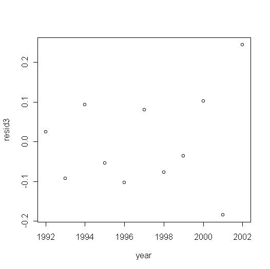
Finally, you can plot the vector of residuals as follows:
resid3<-resid(model3)
plot(year,resid3)

The output will be:

You can also obtain the fitted values and different plots as follows:
fit3<-fitted(model3)  #   This will generate a vector of fitted values for the model 3.
par(mfrow=c(2,2))
plot(model3)      #     This will generate default plots of residuals vs. fitted values, Normal  Q-Q, scale-location, and Cook's distance.
 

Linear Hypothesis Testing

Suppose you want to check whether the variables investment, consumption, and productivity growth matter to GDP growth. In this context, you want to test if those variables matter simultaneously. The best way to check that in R is as follows. First, run a unrestricted model with all variables:
u<-lm(log(gdpgr)~log(invgr)+log(consgr)+log(producgr)+log(unemp)+log(inf))

Then run a restricted model, discarding the variables under test:
r<-lm(log(gdpgr)~log(unemp)+log(inf))

Now you will run a F-test comparing the unrestricted to the restricted model. To do that, you will need to write the F-test function in R, as follows:  (The theory comes from Johston and DiNardo (1997), p. 95, while the R code is a version of Greg Kordas' S code. I've adjusted it for this specific problem.)
 

F.test<-function(u,r)
{
#u is the unrestricted model
k<-length(coef(u))
n<-length(resid(u))
eeu<-sum(resid(u)^2)
#r is the restricted model
kr<-length(coef(r))
eer<-sum(resid(r)^2)
#q is the number of restrictions
q<-k-kr
#F-statistic
Fstat<-((eer-eeu)/q)/(eeu/(n-k))
#P-value
Fprob<-1-pf(Fstat, q, n-k)
list(Fstat=Fstat, Fprob=Fprob)
}
 

After that, you can run the test and obtain the F-statistic and p-value:
F.test(u,r)
$Fstat
[1] 11.40259

$Fprob
[1] 0.01127813

And the conclusion is that you can reject the null hypothesis of joint non-significance at 1.13% level.
 

Saving Operations in R

The simplest way to save commands in R is through the use of a routine. For example, you can append your original routine US90code.txt with the commands you have typed in the R console during the last session. Next time you open this routine, all operations will be registered, and you can access previous outputs by calling the objects you've created.