Econ 508
Econometrics Group
Home | Faculty | Students | Alumni | Courses | Research | Reproducibility | Lab | Seminars | Economics | Statistics | Fame
Applied Econometrics
Econ 508 - Fall 2007

e-Tutorial 19: Duration Models

Welcome. This time we focus on Duration Models (a.k.a. Survival Analysis) in the context of the problem set 5.
 

Downloading your data:

You can download your data from the Econ 508 website (here) and save the file in your preferred directory (I'll save mine as "C:\weco.dat"). Then you open STATA and type:

infile  y sex dex lex kwit tenure censored using "C:\weco.dat"

Drop the first line of the data set containing missing values (due to the labels of variables).

Next you generate the variable lex squared:

gen lex2=lex^2

Then save the file in STATA format (I'll save mine as "C:\weco.dta").

For the purpose of this tutorial, I will use a subsample of the PS5 data set (by dropping lex==12), to demonstrate the main techniques required in the problem set. My results may differ from the original data set. 
 

Question 5:

In STATA, the first thing you need to do is to declare your data set as a survival-time data. You need to identify the "analysis time" variable, and the "failure" variable. The former indicates the duration of the process, while the latter indicates whether the data is censored. In the PS5 data set, "tenure" represents the "analysis-time" variable, i.e., the duration of the process, while "censored" represents the "failure" variable, assuming values of 0 if it is censored, and 1 if it is failure.

stset tenure, failure(censored)

     failure event:  censored ~= 0 & censored ~= .
obs. time interval:  (0, tenure]
 exit on or before:  failure

------------------------------------------------------------------------------
      257  total obs.
        0  exclusions
------------------------------------------------------------------------------
      257  obs. remaining, representing
      213  failures in single record/single failure data
   105811  total analysis time at risk, at risk from t =         0
                             earliest observed entry t =         0
                                  last observed exit t =      5223
 

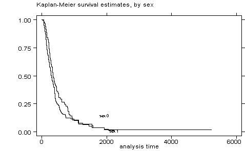
Part (a)

Initially you need to generate the Kaplan-Meier estimator for men and women:

sts graph, by(sex)


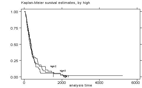
Then you need to stratify the sample into three categories of schooling. In my example I will use lex=13 as the benchmark, but you should adjust for lex=12 as requested by PS5:

gen high=0
replace high=1 if lex==13
replace high=2 if lex>13
sts graph, by (high)


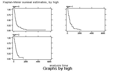
Sometimes the graph is too confused, and it is better to generate separated graphs:

sts graph, by (high) separate


You can also test the equality of survivors as follows:

sts test sex

         failure _d:  censored
   analysis time _t:  tenure

Log-rank test for equality of survivor functions
------------------------------------------------

      |  Events
sex   |  observed       expected
------+-------------------------
0     |        92         105.32
1     |       121         107.68
------+-------------------------
Total |       213         213.00

            chi2(1) =       3.36
            Pr>chi2 =     0.0669

sts test high

         failure _d:  censored
   analysis time _t:  tenure

Log-rank test for equality of survivor functions
------------------------------------------------

      |  Events
high  |  observed       expected
------+-------------------------
0     |       101         101.59
1     |        51          54.91
2     |        61          56.50
------+-------------------------
Total |       213         213.00

            chi2(2) =       0.66
            Pr>chi2 =     0.7206
 

Part (b)

Finally you need to estimate a Cox proportional hazard model, and compare with your results from question 3. You can obtain the Cox PH model as follows:

stcox  sex dex lex lex2

failure _d:  censored
   analysis time _t:  tenure

Iteration 0:   log likelihood = -977.68046
Iteration 1:   log likelihood = -923.63676
Iteration 2:   log likelihood =  -923.3698
Iteration 3:   log likelihood = -923.36976
Refining estimates:
Iteration 0:   log likelihood = -923.36976

Cox regression -- Breslow method for ties

No. of subjects =          257                     Number of obs   =       257
No. of failures =          213
Time at risk    =       105811
                                                   LR chi2(4)      =    108.62
Log likelihood  =   -923.36976                     Prob > chi2     =    0.0000

------------------------------------------------------------------------------
      _t |
      _d | Haz. Ratio   Std. Err.       z     P>|z|       [95% Conf. Interval]
---------+--------------------------------------------------------------------
     sex |   1.772448   .2552638      3.974   0.000       1.336551    2.350507
     dex |   .8976612   .0098688     -9.820   0.000       .8785258    .9172135
     lex |   .4147875   .1430274     -2.552   0.011       .2110152     .815338
    lex2 |   1.034892   .0141125      2.515   0.012       1.007599    1.062925
------------------------------------------------------------------------------

In the output above, a hazard ratio equals one is the benchmark: if the hazard ratio is higher than one, the variable affects positively the hazard; if the hazard ratio is less than one, the variable contributes negatively to the hazard. This can be checked by asking for the coefficients rather than the proportional hazard rates representation of the Cox model:

stcox  sex dex lex lex2, nohr

         failure _d:  censored
   analysis time _t:  tenure

Iteration 0:   log likelihood = -977.68046
Iteration 1:   log likelihood = -923.63676
Iteration 2:   log likelihood =  -923.3698
Iteration 3:   log likelihood = -923.36976
Refining estimates:
Iteration 0:   log likelihood = -923.36976

Cox regression -- Breslow method for ties

No. of subjects =          257                     Number of obs   =       257
No. of failures =          213
Time at risk    =       105811
                                                   LR chi2(4)      =    108.62
Log likelihood  =   -923.36976                     Prob > chi2     =    0.0000

------------------------------------------------------------------------------
      _t |
      _d |      Coef.   Std. Err.       z     P>|z|       [95% Conf. Interval]
---------+--------------------------------------------------------------------
     sex |   .5723616   .1440176      3.974   0.000       .2900922    .8546311
     dex |  -.1079625   .0109938     -9.820   0.000      -.1295101    -.086415
     lex |  -.8799889   .3448208     -2.552   0.011      -1.555825   -.2041525
    lex2 |   .0342972   .0136367      2.515   0.012       .0075698    .0610247
------------------------------------------------------------------------------
 

 Last update: Nov, 30 2007