|
||||||
| Applied
Econometrics
Econ 508 - Fall 2007 e-Tutorial 16: Binary Data Models |
||||||
| Welcome
to the sixteenth issue of e-Tutorial. This time we focus on Binary Data
Models, with special focus to Logit and Probit regressions.
Data You can download your data from the Econ 508 web page (here) and save the file in your preferred directory (I'll save mine as "C:\weco.dat"). Then you open STATA and type: infile y sex dex lex kwit tenure censored using "C:\weco.dat" Drop the first line of the data set containing missing values (due to the labels of variables). Next you generate the variable lex squared:
Then save the file in STATA format (I'll save mine as "C:\weco.dta"). Question 3: On part (a) You need to estimate a simple Logit model: logit(P(quit=1))=(b0 + b1*sex + b2*dex + b3*lex + b4*lex2) In STATA, I will use a subsample of the data set to demonstrate how to obtain the main results. My subsample contains only 257 observations, obtained from dropping lex==12. My results may differ from the original data set in PS5: logit
kwit sex dex lex lex2
This is equivalent to estimate Pr(kwit=1)=exp(xjb)/(1+exp(xjb)). The results above show that, coeteris paribus, workers with higher dexterity are less likely to quit, while males (sex=1) have a bigger tendency to quit than females (sex=0). In other words, positive coefficients contribute to increase the probability of quitting, while negative coefficients, to reduce it. Schooling is not significant in the probability of quitting. To draw a picture of the probability of quitting as a function of years of education, holding everything else constant, you need first to ask for the summary of dexterity for the pooled sample, and then for males and females: summarize dex Variable
| Obs
Mean Std. Dev. Min
Max
summarize dex if sex==0 Variable
| Obs
Mean Std. Dev. Min
Max
summarize dex if sex==1 Variable
| Obs
Mean Std. Dev. Min
Max
Ok. Then you need to calculate the expected probability of quitting, Prob(quit=1)=exp(xib)/(1+exp(xib)). This can be obtained in STATA using the command predict: predict
p
Variable
| Obs
Mean Std. Dev. Min
Max
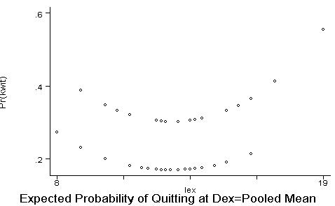
In the table above, kwit is the binary dependent variable, and p is the predicted value of it. But we need to draw a graph of the expected probability of quitting at different years of education, holding the remaining explanatory variables fixed (e.g., at their mean value). Thus, let's ask for the expected value of the probability of quitting conditioned to dexterity being hold at the pooled mean value: replace
dex= 44.6537
In the graph above you see two different curves -- one for male (upper curve) and another for female (lower curve). This happens because we left all explanatory variables constant at their means (in our case, only dex was fixed), but we had to leave sex at its original values (because the average of the dummy variable does not make much sense in this case). On part (b), you are asked to examine better the effect of gender. A first suggestion is to tabulate sen and kwit: tabulate
sex kwit
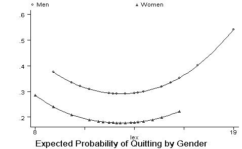
In the table above you can see that 25 out of the existing 119 females in this subsample are quitters, while 45 out of 138 males are quitters. So, the proportion of male quitters (33%) is greater than the proportion of female quitters (21%). Next you can draw graphs of the expected probability of quitting for each gender, using their respective dexterity means. From the results above we know that the dexterity mean for females is 43.90756, and the dexterity mean for males is 45.2971. In STATA, we can ask for the graphs as follows: replace
dex= 43.90756 if sex==0
Besides the graphical analysis, you can also test for the shape of the education effect, by introducing the variables sex*lex and sex*lex2 in the model, and checking their significance. On part (c): You need to evaluate the Logit specification by computing the Pregibon diagnostic. The first thing I recommend is to open the data set again, given that you have replaced dex by its mean values in the construction of the graphs above: use "C:\weco.dta", clear And then re-run the original Logit model: logit kwit sex dex lex lex2 Next you generate the predicted probabilities of quitting, called p, and compute ga (parameter that controls the fatness of tails) and gd (parameter that controls symmetry): predict
p
Finally you run an extended Logit model, including the variables ga and gd: logit
kwit sex dex lex lex2 ga gd
And test their joint significance: test
ga gd
From the results above we can see that the parameters are jointly significantly different than zero. Hence, the Logit model is not a good representation for this data. On part (d): You will provide your
own economic assessment of the problem.
|
||||||