|
||||||||||||||||||||||||||||||||||||||||||||||||||||||||||||||||||||||||||||||||||||||||||||||||||||||||||||||||||
| Applied
Econometrics
Econ 508 - Fall 2007 e-Tutorial 15: Quantile Regression |
||||||||||||||||||||||||||||||||||||||||||||||||||||||||||||||||||||||||||||||||||||||||||||||||||||||||||||||||||
| Welcome
to the fifteenth issue of e-Tutorial. Here you will see basic applications
of Koenker and Bassett (1978) Quantile Regression methodology. The target
is the PS5.
Downloading your data:
infile y sex dex lex kwit tenure censored using "C:\weco.dat" Drop the first line of the data set containing missing values due to the labels in the .txt file. Then save the file in STATA
format (I'll save mine as "C:\weco.dta").
Question 1: On part (a) you are going to run a simple linear regression model: gen
lex2=lex^2
And then you will test the
hypothesis that lex and lex2 are jointly significant:
Note: The test above is based on a quadratic approximation to the likelihood function. The test statistic is the traditional F-statistic. If you wish you can test this hypothesis via likelihood-ratio (LR) test based on the restricted and unrestricted models. The test statistic is now chi-squared: chi2(d0-d1)=-2(L1-L0) where L1 and L0 are the log-likelihood functions, and d1 and d0 the model degrees of freedom, of the constrained (1) and unconstrained (0) regressions respectively. To obtain the test in STATA, proceed as follows: regress
y sex dex lex lex2
Finally you need to test the single hypothesis that lex2 is not significant: regress
y sex dex lex lex2
Don't forget to interpret
the economic meaning of the results.
On part (b) of this question you are asked to plot some graphs using the regression equation of part (a), applying the mean value for dexterity, and 0 or 1 values for gender (each gender has its own curve; you can plot both curves in the same graph). Finally you need to test for different shapes of education. To do that, you can create, for example, the following variables: gen
sexlex=sex*lex
Then regress the models including such variables, and testing their significance: regress
y sex dex lex lex2 sexlex
On part (c)
you need to construct a confidence interval for the optimal level of education
(lex*). You can do that based on the previous tutorials and class notes.
Question 2: For Quantile Regression in R, see Appendix A below. For Quantile Regression in STATA, start here: Part (a): I suggest the following strategy: - Run quantile regressions of the question 1 model at least for the 5th, 25th, 50th, 75th, and 95th quantiles: qreg
y sex dex lex lex2, quant(.05)
Feel free to include as many quantiles as you wish. For example, the output for median regression will be: Median
regression
Number of obs = 683
------------------------------------------------------------------------------
- Next it would be nice if you could construct a table like this (again, feel free to include as many quantiles as you wish): Table 1: Quantile regression estimates for different quantiles
- After you have run the
regression for different quantiles, you can plot the respective curves
for each of these regressions.
Bootstrapped standard errors in STATA: It is recommended the use of bootstrapped standard errors. When you use the bootstrap command, however, you have problems to reproduce the results. To assure reproducibility, fix the seed of the pseudo-random number generator of the bootstrap process as follows: set seed 2 Here the number 2 can be replaced by any other initial value. The reproducibility is assured as long as you use your selected seed whenever you run the quantile regression again. For that matter, you can use the command bsqreg, with say 500 replications: bsqreg y sex dex lex lex2, quant(.50) reps(500) (estimating
base model)
Median
regression, bootstrap(500) SEs
Number of obs = 683
------------------------------------------------------------------------------
For part (b) you need to estimate the mean productivity for each of the quantile regressions you have estimated above. But you should do that according to the years of education. So, first you find the range of years of education: summarize lex Then you construct a table with the estimated productivity according to each year in the range of lex and quantiles: Table 2: Estimated productivity according to quantiles and years of education.
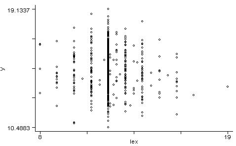
Again, feel free to include more quantiles in your analysis. Please provide an economic discussion of your findings. I suspect that screening the above results between different genders (e.g., a table for males and another for females) would shed light on the hiring decisions. In part (c) you need to interpret the question and try to solve the problem by yourself. The tables above will be very helpful. You can also compare densities according to ranges of years of education, or use any other strategy you think is reasonable. Here are some examples: *Scatter plot of productivity according to years of education: graph y lex
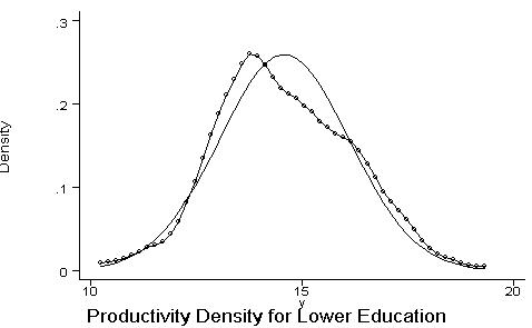
*Kernel density of productivity for individuals with less than 12 years of education (compared with Normal distribution): kdensity y if lex<12, normal title(Productivity Density for Lower Education) xlab ylab
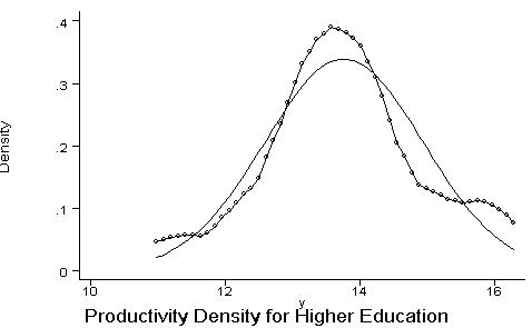
*Compare with the kernel density of productivity for individuals with more than 15 years of education: kdensity y if lex>15, normal title(Productivity Density for Higher Education) xlab ylab
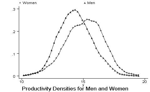
*Finally you can compare the productivity of men and women in a single graph, regardless the years of education: kdensity
y, nogr gen(x fx)
Appendix A: Quantile Regression in R Obviously, you can also perform the Quantile Regression approach in R. There are many advantages in doing that in R. For example, you can generate tables with the coefficients of all requested quantile regressions in a single command. Besides that, you can also plot each regression coefficient (and respective confidence interval) for all quantile regressions in the sample. Moreover, the bootstrapped standard errors can be obtained much faster than in STATA. You can start a simple R session for PS 5 as follows: 1) Infile the data: weco<-read.table("C:/weco.dat", header=T) 2) Extract the variables from the data set: y<-weco$y
Note: If you haven't done so yet, you need to install the package for Quantile Regression, developed by Prof. Koenker, and available at the CRAN web site under the name "quantreg". With your computer connected to the web, you can do that by typing the following commands in the R console: help(install.packages)
3) Before the use of the Quantile Regression toolkit, you need to call the library with the package quantreg: library(quantreg) 4) Run your desired quantile regression. For example, for the median: rq(y~sex+dex+lex+lex2, tau=.5) Call:
Coefficients:
Degrees
of freedom: 683 total; 678 residual
5) To create a table with the main quantiles, you can write: TAB<-table.rq(y~sex+dex+lex+lex2,
method="br")
$a
coefs lower ci limit upper ci limit
, , tau= 0.5
coefs lower ci limit upper ci limit
, , tau= 0.75
coefs lower ci limit upper ci limit
$taus
$method
attr(,"class")
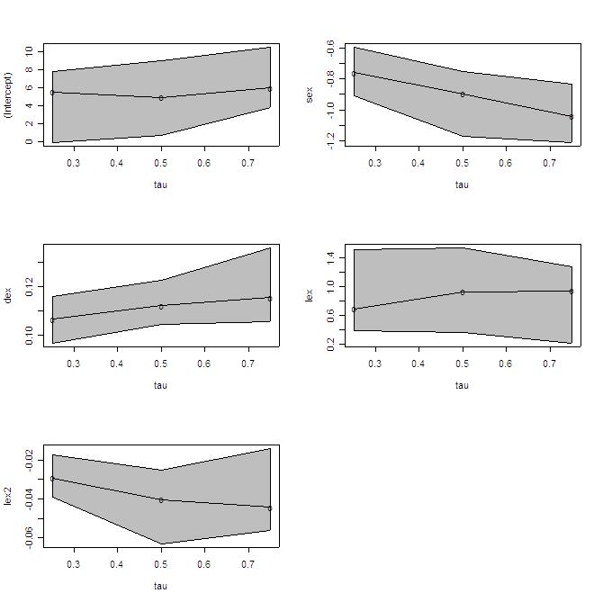
6) To obtain graphs with the coefficients and standard deviations of the main regression quantiles, you can write: plot(TAB)
7) To obtain the standard errors, t-statistics, and p-values for a given quantile regression (e.g., the 10th quantile), you can write: fit1<-rq(y~sex+dex+lex+lex2,
tau=.10)
Call: rq(formula = y ~ sex + dex + lex + lex2, tau = 0.1) Coefficients:
References:
|
||||||||||||||||||||||||||||||||||||||||||||||||||||||||||||||||||||||||||||||||||||||||||||||||||||||||||||||||||