|
||||||||||||||||||||||||||||||
| Applied
Econometrics
Econ 508 - Fall 2007 e-Tutorial 11: Simultaneous Equations Models |
||||||||||||||||||||||||||||||
| Welcome
to the eleventh issue of e-Tutorial. In this issue we introduce simultaneous
dynamic equations and exogeneity (Hausman) tests. I would like to remark
that the theoretical background given in class is essential to proceed
with the computational exercise below. Thus,
I recommend you to consult
Prof. Koenker's Lectures Notes as you go through the tutorial.
The first thing you need
is to download the data sets in ASCII format by clicking in the respecitive
names: system1.dat and system2.dat.
Save them in your preferred location (I'll save mine as "C:/system1.dat"
and "C:/system2.dat"). Then I suggest you to open the files in Notepad
(or another text editor) and type the name of the variable "year" in the
first row, first column, i.e. before the variable "w". Use <Tab> to
separate
the names of variables. Save both files in text format in your favorite
directory (I will save mine as "C:/system1a.txt" and
"C:/system2a.txt",
respectively).
Part 1: For the first part of the
problem set, go to STATA and type:
Next you need to declare
your data as time series:
To obtain a flavor of the data, use the command summarize, detail. To work with time series functions, use previous tutorials. (Supply)
Qt= a1 + a2pt-1+ a3zt
+
ut
Question 1: Here you just need to run
the system above, using OLS:
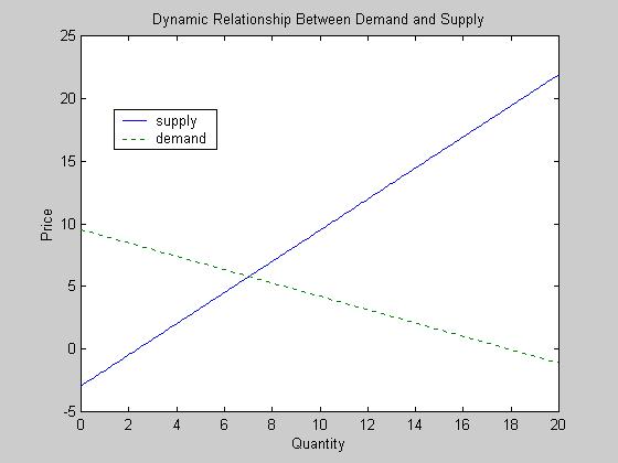
For the graph, first consider the equations in the steady state. Then use the last observations values z and w. Finally plot those two equations in a single cartesian graph. In Matlab, you can do that using the following routine (substitute "yournumber" by the values from the equation system you have run): Q=0:.1:20;
If you don't have access
to Matlab, use any other graphical device or simply draw it by hand. Find
the equilibrium price and quantity. Compare with your graph. Check if there's
convergence in the graph (see Prof. Koenker class notes).
Question 2: Here I suggest you to construct a table as follows:
The values at n=0 come from
the last observation in the data set. After that, z and w stay fixed. To
find p(n=1), you need first to calculate the forecast of Q(n=1). Use the
system of equations you have estimated in question 1. Do the same for p(n=i),
i=2,..., 20. Find prices and quantities of equilibrium.
Question 3: A) Explaining the effects of autocorrelation: The problem asks you to explain why L.p cannot be considered exogenous. Please also explain the consequences of applying OLS estimators in the presence of autocorrelated disturbances. B) Testing for the presence of autocorrelation: see e-Tutorial 10. C) Correcting the Model:
see e-Tutorial 10.
Question 4: Here you can use the Hausman specification test you have saw in Lecture 11. Make sure to explain the null and the alternative hypothesis, and describe how the test is computed. The choice of instruments is crucial: you need to select instruments that are exogenous, orthogonal to errors, but correlated with included variables. In STATA, you can calculate the Hausman test as follows: *2SLS
with full set of instruments:
*2SLS
with reduced set of instruments:
*Hausman
Specification Test:
After you obtain your
test statistic Delta - a scalar, you should compare it with a Chi-squared
(1). The degrees of freedom correspond to the number of dubious variables,
i.e., the number of variables included as instruments in the first equation,
but not in the second equation. Compare your results with the command hausman
in STATA.
Part 2: For the second part of the
problem set, go to STATA and type:
Next you need to declare
your data as time series:
To obtain a flavor of the data, use the command summarize, detail. To work with time series functions, use previous tutorials. (Supply)
Qt= a1 + a2pt+ a3pt-1
+
a4zt + ut
The variable p1 in the data
set was created to substitute the lag of p, so you don't have to
loose any observation.
Question 5: Here you just need to compare the OLS estimators with the 2SLS estimators for the whole system: *Supply
*Demand:
As an econometrician, draw
your analysis on the results above. Check signs, significance, and economic
sense of the results.
Question 6. This question is a simple hyptohesis testing exercise. Nevertheless, you don't know if you should test using OLS or 2SLS. The results might be different according to the model. So, I suggest you to implement a Hausman-Wu test, similar to the one you did in question 4, but considering a simple OLS regression versus a 2SLS. You decide your instruments. To implement the test, follow the commands in question 4, adjusting for the OLS equation. Based on your diagnostic, choose the best model (OLS or 2SLS), and type in STATA the following commands: *Is
the long-run supply response to change in price equals 1?
Optional: Checking if the errors are correlated in a system of equations: Sometimes is useful to know whether the errors of the supply equation are correlated with the errors of the demand equation. For example, using 2SLS methods: *Supply:
If you find the residuals
are correlated, maybe it is because some of the variables are not exogenous.
Then you can proceed with the Hausman test to verify who is not exogenous
among the instruments.
|
||||||||||||||||||||||||||||||