|
||||||
| Applied
Econometrics
Econ 508 - Fall 2007 e-Tutorial
10:
|
||||||
| Welcome
to the tenth issue of e-Tutorial. The first part of the tutorial is useful for the first part of problem set 3.
It will
help you to understand details of Granger and Newbold (1974).
This time I focus on Monte
Carlo Simulation and Nonlinear Regression. I introduce these two topics
in form of examples connected to Econ 508 syllabus. For the Monte Carlo,
I use the Granger-Newbold experiment on spurious regression as an example.
For the Nonlinear Regression, I give examples of how to correct autoccorelated
errors (Cochrane-Orcutt and NLS).
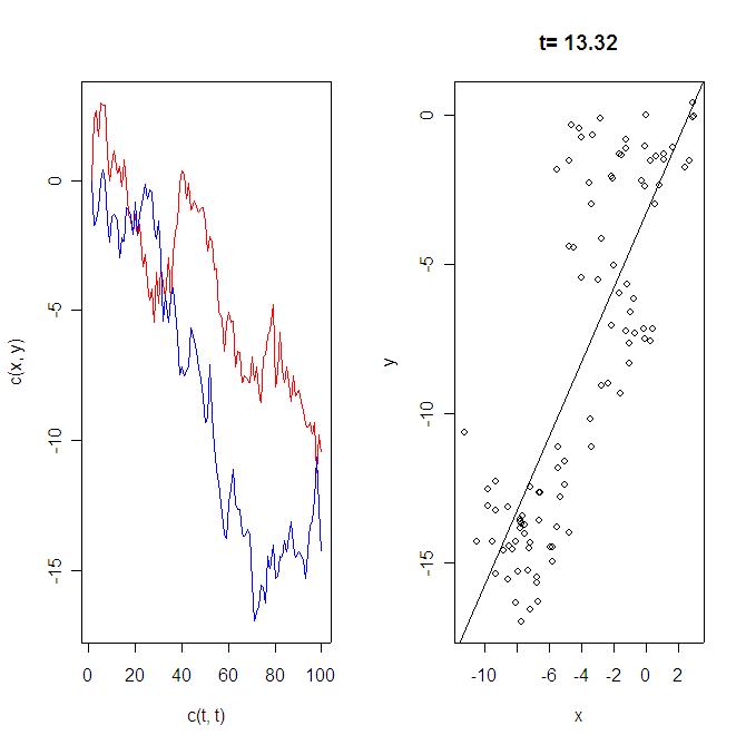
Monte Carlo Simulation: In the Granger-Newbold (1974) experiment, the econometrician has a bivariate model as follows: x(t) = x(t-1) + v(t) u(t) and v(t) are identically indepedently distributed. Hence, each variable has a unit root, and their differences, y(t)-y(t-1)=u(t) and x(t)-x(t-1)=v(t), are pure noise. However, as you regress y(t) on x(t), you may obtain significant linear relationship based on conventional OLS and t-statistics, contrary to your theoretical expectations. Let's replicate the experiment.
The algorithm is as follows:
This corresponds to a single loop of the experiment, but it is already enough to show the nuisance. If you wish, you can go ahead and repeat this loop B times and check how many times you get significance. Below I provide the routine
for one loop of the experiment in R, designed by Prof. Koenker, which can
also also be accessed at the Econ
508 web page, Routines.
R Code: #Start
copying here:
An the output will be:
Because you are running
regressions on random numbers, the experiments provide different results
as you run each of them. Nevertheless, as many times you run as more convinced
you will be that in a large proportion of the cases the t-statistics will
be very significant, meaning that you have spurious regression in many
cases.
STATA Code: Below I also provide the respective routine for one loop of the experiment using STATA, which can also also be accessed at the Econ 508 web page, Routines, under the name gn.do. . do "C:\Documents and Settings\econ472\WWW\gn.do" . clear all .
set obs 100
. gen t=_n . gen u=invnorm(uniform()) .
gen y=u if t==1
.
replace y=y[_n-1]+u if t>1
. gen v=invnorm(uniform()) .
gen x=v if t==1
.
replace x=x[_n-1]+v if t>1
. regress y x
Source | SS
df MS
Number of obs = 100
------------------------------------------------------------------------------
.
predict fit
.
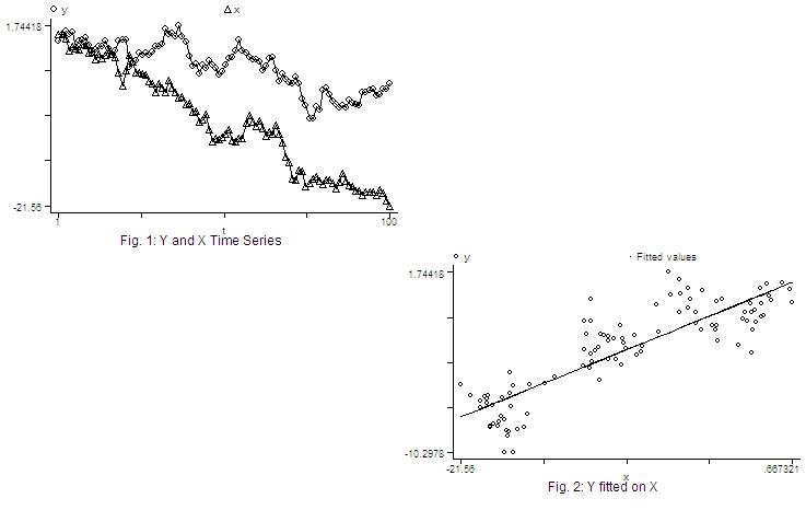
graph y x t, c(ll) title("Fig. 1: Y and X Time Series") saving (fig1, replace
.
graph y fit x, c(.l) s(o.) title ("Fig. 2: Y fitted on X") saving (fig2,
repl
. graph using, saving (null, replace) . graph using fig1 null null fig2, saving (gn, replace) .
.
Nonlinear Regression: I explain nonlinear regression thorugh the data sets of the problem set 3. You can download them in ASCII format by clicking in the respecitive names: system1.dat and system2.dat. Save them in your preferred location (I'll save mine as "C:/system1.dat" and "C:/system2.dat"). Then I suggest you to open the files in Notepad (or another text editor) and type the name of the variable "year" in the first row, first column, i.e. before the variable "w". Use <Tab> to separate the names of variables. Save both files in text format in your favorite directory (I will save mine as "C:/system1a.txt" and "C:/system2a.txt", respectively). The problem: Suppose you have the following equation: Qt= a1 + a2pt-1+ a3zt + ut and you suspect the errors are autocorrelated. The first you need to explain why pt-1 cannot be considered exogenous. Please also explain the consequences of applying OLS estimators in the presence of autocorrelated disturbances. Testing for the presence of autocorrelation: Next you need to test for the presence of autocorrelation. You already saw a large menu of options for that. Here I suggest the use of the Breusch-Godfrey test: Background:
ut= b1ut-1 + b2ut-2 + ...+ bpzt-p + et You wish to test whether any of the coefficients of lagged residuals is different than zero. Your null hypothesis is no autocorrelation, i.e., b1=b2=...=bp=0. For example, to test for the presence of autocorrelation using 1 lag (AR(1)), do as follows: *Run an OLS in your original
equation:
*Obtain the estimated residuals:
* Regress the estimated
residuals on the explanatory variables of the original model and lag of
residuals:
*From the auxilliary regression
above, obtain the R-squared and multiply it by number of included observations:
This nR2
may be compared with a Chi-squared(1) distribution. If you need
to test autocorrelation using p lags, compare your statistic with a Chi-squared
(p). Hint: Be parsimonious - don't push the data too much, and try
to use at most 4 lags. However, observe that the first lag is enough to
detect autocorrelation here..
Correcting the Model: After you detect autocorrelation, you need to correct it. Let's see how it works in our data. Suppose we have obtained the following AR(1) autocorrelation process: (1)
Qt= a1
+ a2pt-1+ a3zt
+
ut
where et is white noise. Now generate the lag of equation (1): (3) Qt-1= a1 + a2pt-2+ a3zt-1 + ut-1 and substitute (3) into the equation (2): (4) ut= b1(Qt-1- a1 - a2pt-2- a3zt-1) + et Substituting equation (4) into the equation 1 will give you an autocorrelation-corrected version of your original equation: (5)
Qt= a1
+ a2pt-1+ a3zt
+
ut
This corrected model contain multiplicative terms in the coefficients, and therefore need to be re-estimated by Non-linear Least Squares (NLS). (Hint: Here the coefficients are non-linear. So, you need NLS. But if instead of the coefficients, the variables were non-linear, than you could have used linear models like OLS.) In STATA you should write the following program to run this model: program
define nlg
In the program above:
Ok. After you have created the program g, you need to run it. Attempt to one detail: the program does not work in the presence of missing values. As you have generated lags, you also have lost the first 2 observations. Thus, you need to restrict your optimization problem to the existing observations. nl
g Q if year>1960.25
That is it. The output should give you the requested elements to calculate equation (5) - the model adjusted for autocorrelation. Similar result can be obtained through the Cochrane-Orcutt method. In STATA, you can obtain that as follows: prais Q L.p z, corc This will give you the adjusted
coefficients of each explanatory variable, plus the Durbin-Watson statistic
before and after the correction. Compare the Cochrane-Orcut results
with the NLS results, and see how similar they are. Then compare both NLS
and Cochrane-Orcutt with the naive OLS from question 1, and draw your conclusions.
References
|
||||||