e-Tutorial 1: A Brief Introduction to STATA

Accessing Stata
The statistical package Stata can be found at the OCSS (Office of Computing and Communications for Social Sciences) lab, located at the 212 Lincoln Hall. Also, you can find Stata at the Foreign Languages Building (FLB) (room G8). It is also available at the Econometrics Lab, DKH, for students enrolled in the Econometrics field or other classes that require lab experiments.

STATA has an extraordinary set of reference books, and by this reason some students may be interested in purchasing the package. In those cases, the best strategy is to form a group of students and make a special order to STATA Inc. For Econ 508 purposes, however, the weekly edition of e-Tutorial will bring all necessary information to solve the homework.

Downloading Data
The first step required to solve the homework is to download the respective data sets. Usually the data will be posted in the  ASCII or text formats. In order to work with the data, I suggest the following steps:
a) Go to the web page containing the data, and save it in a floppy disk or a hard drive. If the latter is chosen, I suggest you create a directory exclusively dedicated to Econ508 materials.
b) After saving, go to STATA and infile the data in its original format.
c) Finally, save the data in the format .dta, adopted by STATA.

Example - The U.S. Economy in the 1990s
Let's start with an analysis of the performance of the U.S. economy during the 1990s. I have collected annual data on GDP growth, GDP per capita growth, private consumption growth, investment growth, manufacturing labor productivity growth, unemployment rate, and inflation rate. The first two variables can be seen as dependent variables, and you should test whether they are close substitutes or the population size has dramatically changed during this period. Consumption, investment, and productivity can be seen as factors that enhance GDP growth, and therefore you should expect positive covariates for those variables. Finally, unemployment and inflation rates are intrinsically correlated, and you should check whether any (or both) can be included in our simplistic growth model.

Please click here to access the data in a text format. After data, save as recommended, and go to the Stata Command window. There, please type the following command:
infile year gdpgr consgr invgr unemp gdpcapgr inf producgr using "a:\US90.txt"

(I assumed that you have saved the data set in a floppy disk and the file has .txt extension. If the file has a .raw format or you wish to save it in a different location, just repeat the command above doing the respective adjustments (i.e., including your preferred directory and changing file extension). For ASCII data with .raw format, you can omit the extension. E.g.:
infile year gdpgr consgr invgr unemp gdpcapgr inf producgr using "c:\Econ472\US90"

In the commands above, the term "ïnfile" refers to the action executed by Stata, the terms "gdpgr, ..., producgr" correspond to the name of the respective variables according to the order they appear in the data set, and the rest of the command describes the location you have chosen to save the downloaded data. After that, you can visualize your data using the button "Data Editor" in the toolbar. The final step is to save the file in a Stata format, with the extension .dta. Now you are ready to work with your data!!

Basic Operations
A useful way to explore your data is checking the main statistics of each variable. For example, in the Stata Command window you can obtain the minimum, maximum, arithmetic mean, and standard deviation of each variable in your data set by typing
summarize

Variable |     Obs        Mean   Std. Dev.       Min        Max
---------+-----------------------------------------------------
    year |      11        1997   3.316625       1992       2002 
   gdpgr |      11    3.463636   1.050974        1.5          5 
  consgr |      11    3.645455    1.03476        2.4        5.3 
   invgr |      11    6.954545   2.408885        3.3       10.7 
   unemp |      11    5.327273   1.125247          4        7.5 
gdpcapgr |      11    2.490909   1.048289         .7        4.2 
     inf |      11    2.590909   .5204893        1.5        3.4 
producgr |      11    4.309091   1.590883        1.9        7.2 
 

If you also wish to know the behavior along the percentiles, type
summarize, detail

If you are only interested in a single variable, just include its name after the command
summarize gdpgr, detail

If you are only interested in a subset of your data, you can inspect it using filters. E.g., if you are only interested in the years of the Clinton administration, you type
summarize if year>=1993 & year<=2000

And then you can contrast that period with the family Bush administrations
summarize if year<1993 | year>2000

You may also check all years but the election years, to avoid political cycles:
summarize if year~= 2000 & year~=1996 & year~=1992

At this point you have already noticed the main logical operators in Stata: 
>=    means    "greater or equal", 
<=    means    "less or equal", 
&      means    "and", 
|       means    "or". 
The arithmetic operators are as usual (+, -, *, /). And to create a new variable using them, you can do as follows: Suppose you wish to know how close the GDP growth is to the GDP per capita growth. So, you create a ratio of those two variables, and check it:
generate gdpratio= gdpgr/ gdpcapgr
summarize gdpratio, detail

The same procedure can be done to obtain traditional transformations, such as
squares:       gen produc2=producgr^2
square roots:     gen infroot=sqrt(inf)
exponential:      gen expgdpgr=exp(gdpgr)
natural logs:     gen logunemp=log(unemp) or simply gen lnunemp=ln(unemp)
base 10 logs:     gen log10inf=log10(inf)

A final remark is that you should choose a name for the generated variable with at most 8 characters, otherwise the system will give an error message. Nevertheless, you can always describe your variables in more details using the commands label or notes. Last, but not least, the Help toolbar contains short but useful information on the main commands. It does not hurt visit it once in a while...
 

Exploring Graphical Resources
Suppose now you want to check the relationship among variables. For example, you want to see how much consumption and investment are correlated with GDP (all variables in growth rates). The command for that is:
graph gdpgr consgr invgr year

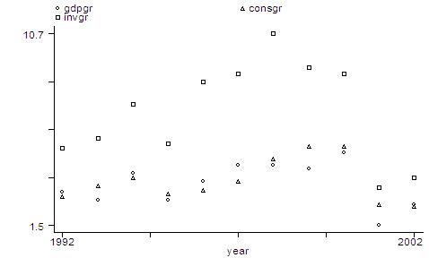
The output is a scatter of points for each series, with the investment series being relatively higher than the other two series. If you are more interested on the dynamics of the series than in the levels, you can re-scale the graph and connect the points. The command is as follows:
graph gdpgr consgr invgr year, rescale c(lll)

In the command above, "rescale" allows the shift on the series, and "c(lll)" connects the points using lines for each series. Many other graph types are available in STATA, and you can explore them as necessary. In this brief intro, the following commands will be useful:

* to extract the symbols on the series:
graph gdpgr consgr invgr year, rescale c(lll) symbol(iii)

* to give a title to the graph: 
graph gdpgr consgr invgr year, c(lll) b1(Figure 1. GDP, Consumption and Investment) b2(year) l2(growth rate)

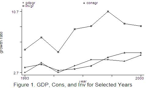
* to plot only specific ranges: 
graph gdpgr consgr invgr year if year>=1993 & year<=2000, c(lll) b1(Figure 1. GDP, Cons, and Inv for Selected Years) b2(year) l2(growth rate)

Finally, you can combine graphs in a single figure. For example, suppose you would like to obtain a graphical diagnostic on the relationship between GDP and consumption growth rates, GDP and investment growth rates, GDP and productivity growth rates, and revisit the relation between unemployment and inflation rates. The commands to do that are as follows:
graph  gdpgr  consgr, saving(part1)
graph  gdpgr  invgr, saving(part2)
graph  gdpgr  producgr, saving(part3)
graph  unemp  inf, saving(part4)
graph  using  part1  part2  part3  part4,  margin(10)

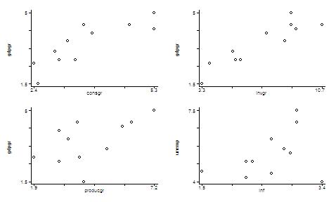
Through the commands above, you generated and saved four individual graphs, and plotted them into a single figure. The command margin(10) means that you are requiring a space between each pair of graphs about 10% of the whole picture. This is indeed a very useful tool to check pair wise correlation among variables, before you run a regression.
 

Linear Regression
As remarked above, before running a regression, it is recommended to check the cross correlation among covariates. You can do that graphically (see above) or using the following simple command:
correlate gdpgr gdpcapgr consgr invgr producgr unemp inf
(obs=11)

         |    gdpgr gdpcapgr   consgr    invgr producgr    unemp      inf
---------+---------------------------------------------------------------
   gdpgr |   1.0000
gdpcapgr |   0.9890   1.0000
  consgr |   0.8394   0.8347   1.0000
   invgr |   0.9097   0.8841   0.8270   1.0000
producgr |   0.5708   0.6003   0.7050   0.5238   1.0000
   unemp |  -0.3035  -0.4143  -0.4761  -0.3684  -0.5336   1.0000
     inf |  -0.1012  -0.1230  -0.1198  -0.3090  -0.0832   0.3590   1.0000

From the matrix above you can see, for example, that GDP and GDP per capita growth rates are closely related, but each of them has a different degree of connection with unemployment rates. In fact, GDP per capita growth rates present higher negative correlation with unemployment rates (41.43%) than total GDP growth rates do (30.35%). Inflation and unemployment rates present a reasonable degree of positive correlation (35.90%).

Now you start with simple linear regressions. For example, let's check the individual regressions of GDP with consumption and investment growth rates:
regress gdpgr consgr
regress gdpgr invgr

The output will be

. regress  gdpgr consgr

  Source |       SS       df       MS                  Number of obs =      11
---------+------------------------------               F(  1,     9) =   21.46
   Model |  7.78197201     1  7.78197201               Prob > F      =  0.0012
Residual |  3.26348251     9  .362609168               R-squared     =  0.7045
---------+------------------------------               Adj R-squared =  0.6717
   Total |  11.0454545    10  1.10454545               Root MSE      =  .60217

------------------------------------------------------------------------------
   gdpgr |      Coef.   Std. Err.       t     P>|t|       [95% Conf. Interval]
---------+--------------------------------------------------------------------
  consgr |   .8525216   .1840263      4.633   0.001       .4362251    1.268818
   _cons |   .3558076   .6949943      0.512   0.621      -1.216379    1.927994
------------------------------------------------------------------------------

. regress  gdpgr  invgr

  Source |       SS       df       MS                  Number of obs =      11
---------+------------------------------               F(  1,     9) =   43.22
   Model |  9.14164404     1  9.14164404               Prob > F      =  0.0001
Residual |  1.90381048     9  .211534498               R-squared     =  0.8276
---------+------------------------------               Adj R-squared =  0.8085
   Total |  11.0454545    10  1.10454545               Root MSE      =  .45993

------------------------------------------------------------------------------
   gdpgr |      Coef.   Std. Err.       t     P>|t|       [95% Conf. Interval]
---------+--------------------------------------------------------------------
   invgr |   .3969137   .0603774      6.574   0.000       .2603305    .5334969
   _cons |   .7032821   .4422039      1.590   0.146      -.2970526    1.703617
------------------------------------------------------------------------------

Please note that you don't need to include the intercept, because STATA automatically includes it. In the output above you have the main regression diagnostics (ANOVA, adjusted R-squared, t-statistics, sample size, etc.). The same rule apply to multiple linear regressions. For example, suppose you want to find the main sources of GDP growth. You type:
regress gdpgr consgr invgr producgr unemp inf

And the output will be:

. regress  gdpgr  consgr  invgr  producgr  unemp  inf

  Source |       SS       df       MS                  Number of obs =      11
---------+------------------------------               F(  5,     5) =    7.27
   Model |  9.70924721     5  1.94184944               Prob > F      =  0.0242
Residual |  1.33620731     5  .267241462               R-squared     =  0.8790
---------+------------------------------               Adj R-squared =  0.7581
   Total |  11.0454545    10  1.10454545               Root MSE      =  .51695

------------------------------------------------------------------------------
   gdpgr |      Coef.   Std. Err.       t     P>|t|       [95% Conf. Interval]
---------+--------------------------------------------------------------------
  consgr |   .1822094   .3605194      0.505   0.635      -.7445351    1.108954
   invgr |   .3448859   .1338048      2.578   0.050       .0009296    .6888422
producgr |   .0490201   .1547288      0.317   0.764      -.3487228    .4467631
   unemp |   .0551669   .1897954      0.291   0.783      -.4327176    .5430514
     inf |   .3019558    .372596      0.810   0.455      -.6558326    1.259744
   _cons |  -.8865854   1.492931     -0.594   0.578      -4.724287    2.951116
------------------------------------------------------------------------------

In the example above, despite we have a high adjusted R-squared, most of the covariates are not significant at 5% level (actually, only the investments coefficient is significant at this level). There may be many problems in the regression above. On the Econ 508 classes you will learn how to solve most of those problems, including how to select the best specification for a model.

You can also run a log-linear regression after transforming each variable into a natural log scale. To do so, you type:
gen lngdpgr=ln(gdpgr)
gen lnconsgr=ln(consgr)
gen lninvgr=ln(invgr)
gen lnproduc=ln(producgr)
gen lnunemp=ln(unemp)
gen lninf=ln(inf)
regress lngdpgr lnconsgr lninvgr lnproduc lnunemp lninf

  Source |       SS       df       MS                  Number of obs =      11
---------+------------------------------               F(  5,     5) =    7.19
   Model |  1.07467131     5  .214934262               Prob > F      =  0.0247
Residual |  .149400242     5  .029880048               R-squared     =  0.8779
---------+------------------------------               Adj R-squared =  0.7559
   Total |  1.22407155    10  .122407155               Root MSE      =  .17286

------------------------------------------------------------------------------
 lngdpgr |      Coef.   Std. Err.       t     P>|t|       [95% Conf. Interval]
---------+--------------------------------------------------------------------
lnconsgr |    .114882   .4666926      0.246   0.815       -1.08479    1.314554
 lninvgr |    .779761   .3081229      2.531   0.052      -.0122942    1.571816
lnproduc |   .0950277   .1935535      0.491   0.644      -.4025174    .5925728
 lnunemp |   .2009322   .3716735      0.541   0.612      -.7544849    1.156349
   lninf |   .1184624   .2785439      0.425   0.688      -.5975574    .8344822
   _cons |  -.9912522    .787582     -1.259   0.264      -3.015796    1.033292
------------------------------------------------------------------------------
 

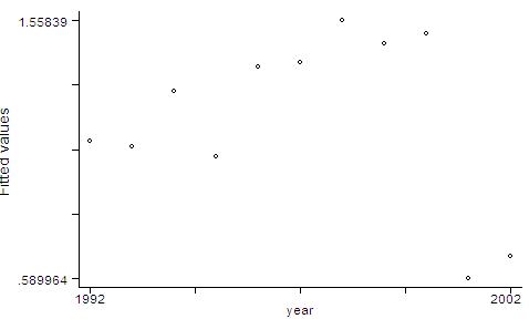
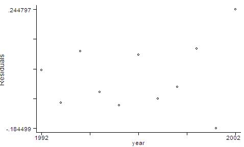
Finally, you can generate predicted values of the dependent variable and of the residuals, and plot them: 
predict lngdpfit
graph lngdpfit year

predict lngdpres, resid
graph lngdpres year

Linear Hypothesis Testing
After running the regressions above, we can proceed with tests of linear hypothesis on the covariates. For example, suppose you would like to be sure that investment growth "matters" to GDP growth. **(Please recall that you are no longer performing causality tests, but only detecting whether the two variables are correlated. Through the Econ 508 classes, you will learn how to perform causality tests.)**  Thus, you proceed with:
test lninvgr

And the output will be:
 ( 1)  lninvgr = 0.0

       F(  1,     5) =    6.40
            Prob > F =    0.0525
 

You just performed a F-test for the null hypothesis of lninvgr=0 against the alternative of lninvgr ~= 0. The computed F-statistic is the squared of the popular t-statistic. The result means that investment growth rates (in logs) are significantly different than zero at 5.25%  level, and therefore they contribute to explain the variation in GDP growth rates (in logs).

To test the joint significance of two or more covariates, you type:
test lninvgr lnconsgr lnproduc

And the output will be:
  ( 1)  lninvgr  = 0.0
 ( 2)  lnconsgr = 0.0
 ( 3)  lnproduc = 0.0

       F(  3,     5) =   11.40
            Prob > F =    0.0113
Here you are testing the null hypothesis that all covariates are zero against the alternative hypothesis that at least one of them is different than zero. The result shows that we cannot accept the null at 1.13% of significance, i.e., some of them are significantly different than zero at this level. So, some of them "matter" in explaining the variation in GDP growth rates (logs) along the years.

You could also extend your tests and check the equality of covariates. For example, suppose you would like to know if investments and consumption have similar coefficients:
test lninvgr=lnconsgr

The output will be:
 ( 1) - lnconsgr + lninvgr = 0.0

       F(  1,     5) =    0.79
            Prob > F =    0.4143

This is similar to test whether their difference is zero (null hypothesis) or different than zero (alternative). The conclusion is that, at 5% significance level, we cannot reject the null hypothesis of similarity.