Lecture 8 Figure 1: R code

                    #Edit the function predict.arima0 substituting the following two lines:
        #data <- data - xreg %*% coefs[-(1:narma)]
        #xm <- drop(newxreg %*% coefs[-(1:narma)])
        #by these two lines:
        #data <- data - as.matrix(xreg) %*% coefs[-(1:narma)]
        #xm <- drop(as.matrix(newxreg) %*% coefs[-(1:narma)])

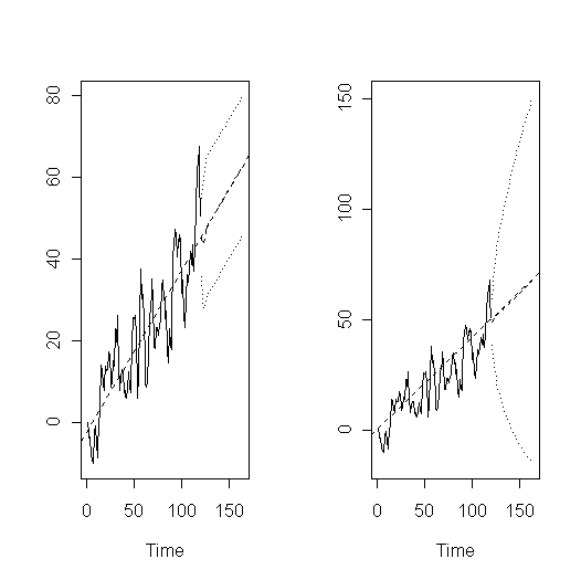
        # Figures to illustrate the difference between forecasting in Trend
        # Stationary and Unit Root Models for Lecture 8 of 508
        u <- rnorm(120)
        s <- 1:120
        y <- .3*s+5*filter(u,c(.95,-.1),"recursive",init=rnorm(2))
        fit0 <- arima0(y,order=c(2,0,0),xreg=s)
        fit1 <- arima0(y,order=c(2,1,0),xreg=s,include.mean=T)
        fore0 <- predict(fit0,n.ahead=44,newxreg=121:164)
        fore1 <- predict(fit1,n.ahead=44,newxreg=121:164)
        postscript("fig1.ps",horizontal=F,width=6.0,height=4)
        par(mfrow=c(1,2))
        ts.plot(y,fore0$pred,fore0$pred+2*fore0$se, fore0$pred-2*fore0$se,
        gpars=list(lty=c( 1,2,3,3)))
        abline(fit0$coef[3:4],lty=2)
        ts.plot(y,fore1$pred,fore1$pred+2*fore1$se, fore1$pred-2*fore1$se,
        gpars=list(lty=c( 1,2,3,3)))
        abline(c(0,fit1$coef[3]),lty=2)

        dev.off()